Wireless Network Experiment Three: Queuing Theory
ABSTRACT
This experiment is designed to learn the fundamentals of the queuing theory. Mainly about the M/M/S and M/M/n/n queuing MODELS.
KEY WORDS: queuing theory, M/M/s, M/M/n/n, Erlang B, Erlang C. INTRODUCTION
A queue is a waiting line and queueing theory is the mathematical theory ofwaiting
lines.More generally, queueing theory is concerned with the mathematical modeling and analysisof systems that provide service to random demands. Incommunication networks, queues are encountered everywhere. For example, theincoming data packets are randomly arrived and buffered, waiting for the routerto deliver. Such situation is considered as a queue.
A queueing model is an abstract description of such a system. Typically, a queueing model represents (1) thesystem's physical configuration, by specifying the number and arrangement of theservers, and (2) the stochastic nature of the demands, by specifying the variabilityin the arrival process and in the service process.
The essence of queueing theory is that it takes into account the randomness ofthe arrival process and the randomness of the service process. The most commonassumption about the arrival process is that the customer arrivals follow a Poisson process, where the times between arrivals are exponentially distributed. Theprobability of the exponential distribution function
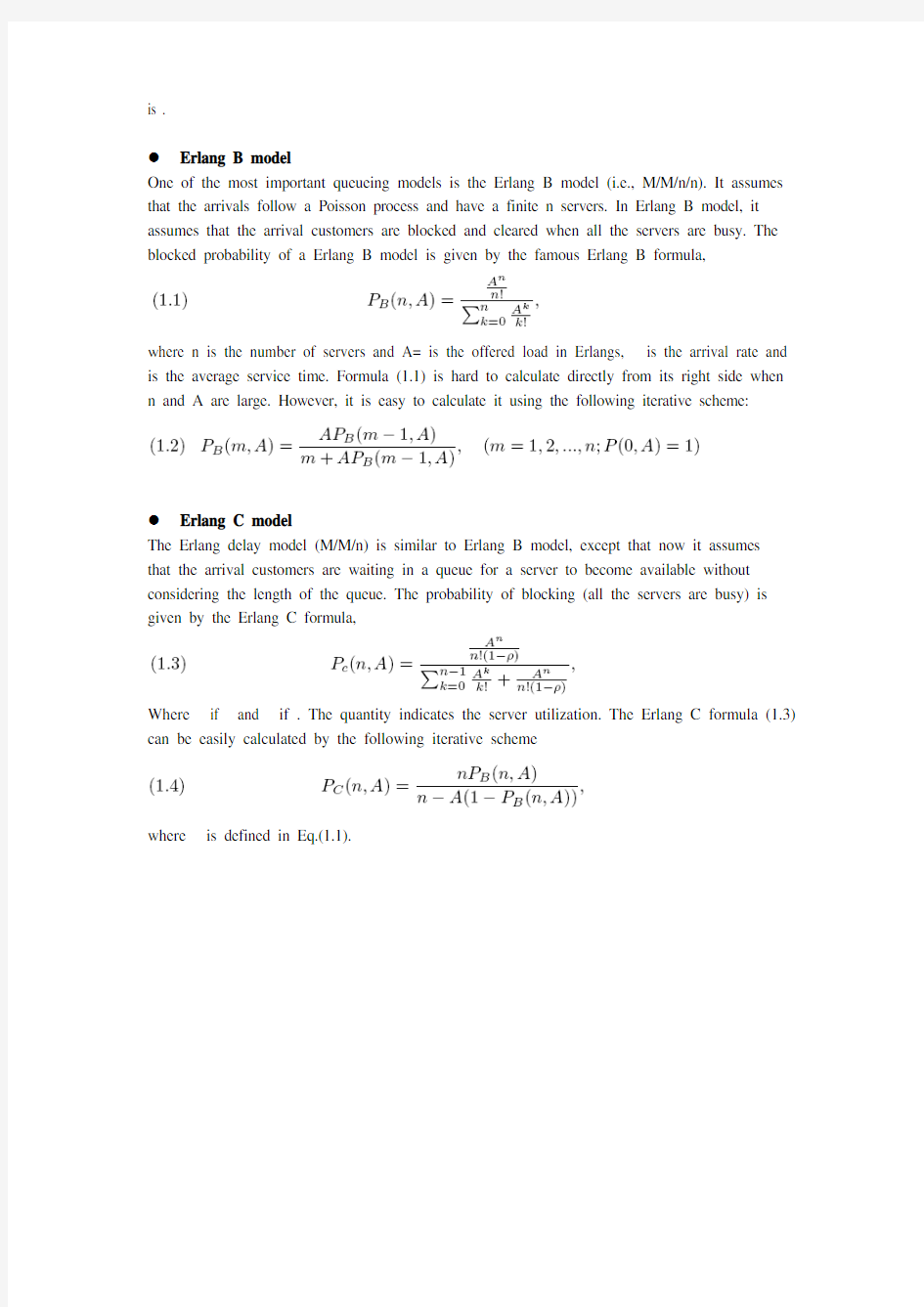
●Erlang B model
One of the most important queueing models is the Erlang B model (i.e., M/M/n/n).It assumes that the arrivals follow a Poisson process and have a finite n servers.In Erlang B model, it assumes that the arrival customers are blocked and clearedwhen all the servers are busy. The blocked probability of a Erlang B model is givenby the famous Erlang B formula,
w here n is the number of servers and A= is the offered load in Erlangs, is the arrival rate andis the average service time. Formula (1.1) is hard tocalculate directly from its right side when n and A are large. However, it is easy tocalculate it using the following iterative scheme:
●Erlang C model
The Erlang delay model (M/M/n) is similar to Erlang B model, except that nowit assumes that the arrival customers are waiting in a queue for a server to becomeavailable without considering the length of the queue. The probability of blocking(all the servers are busy) is given by the Erlang C formula,
Where if and if . The quantityindicates the serverutilization. The Erlang C formula (1.3) can be easily calculated by the followingiterative scheme
where is defined in Eq.(1.1).
DESCRIPTION OF THE EXPERIMENTS
https://www.doczj.com/doc/172164936.html,ing the formula (1.2), calculate the blocking probability of the ErlangB model.
Draw the relationship of the blocking probability PB(n,A) and offered traffic A with n = 1,2, 10, 20, 30, 40, 50, 60, 70, 80, 90, 100. Compareit with the table in the text book (P.281, table 10.3).
From the introduction, we know that when the n and A are large, it is easy to calculate the blocking probability using the formula 1.2 as follows.
it use the theory of recursion for the calculation. But the denominator and the numerator of the formula both need to recurs() when doing the matlab calculation, it waste time and reduce the matlab calculation efficient. So we change the formula to be :
Then the calculation only need recurs once time and is more efficient.
The matlab code for the formula is: erlang_b.m
%**************************************
% File: erlanb_b.m
% A = offered traffic in Erlangs.
%n = number of truncked channels.
% Pb is the result blocking probability.
%**************************************
function [ Pb ] = erlang_b( A,n )
if n==0
Pb=1; % P(0,A)=1
else
Pb=1/(1+n/(A*erlang_b(A,n-1))); % use recursion "erlang(A,n-1)" end
end
As we can see from the table on the text books, it uses the logarithmcoordinate, so we also use the logarithm coordinate to plot the result. We divide the number of servers(n) into three parts, for each part we can define a interval of the trafficintensity(A) based on the figure on the text books :
1. when 0 2. when 10 3. when 30 For each part, use the “erlang_b”function to calculate and then use “loglog”function to figure the logarithm coordinate. The matlab code is : %***************************************** % for the three parts. % n is the number servers. % A is the traffic indensity. % P is the blocking probability. %***************************************** n_1 = [1:2]; A_1 = linspace(0.1,10,50); % 50 points between 0.1 and 10. n_2 = [10:10:20]; A_2 = linspace(3,20,50); n_3 = [30:10:100]; A_3 = linspace(13,120,50); %***************************************** % for each part, call the erlang_b() function. %***************************************** for i = 1:length(n_1) for j = 1:length(A_1) p_1(j,i) = erlang_b(A_1(j),n_1(i)); end end for i = 1:length(n_2) for j = 1:length(A_2) p_2(j,i) = erlang_b(A_2(j),n_2(i)); end end for i = 1:length(n_3) for j = 1:length(A_3) p_3(j,i) = erlang_b(A_3(j),n_3(i)); end end %***************************************** % use loglog to figure the result within logarithm coordinate. %***************************************** loglog(A_1,p_1,'k-',A_2,p_2,'k-',A_3,p_3,'k-'); xlabel('Traffic indensity in Erlangs (A)') ylabel('Probability of Blocking (P)') axis([0.1 120 0.001 0.1]) text(.115, .115,'n=1') text(.6, .115,'n=2') text(7, .115,'10') text(17, .115,'20') text(27, .115,'30') text(45, .115,'50') text(100, .115,'100') The figure on the text books is as follow: We can see from the two pictures that, they are exactly the same with each other except that the result of the experiment have not considered the situation with n=3,4,5,…,12,14,16,18. https://www.doczj.com/doc/172164936.html,ing the formula (1.4), calculate the blocking probability of the Erlang C model. Draw the relationship of the blocking probability PC(n,A) and offered traffic A with n = 1,2, 10, 20, 30, 40, 50, 60, 70, 80, 90, 100. From the introduction, we know that the formula 1.4 is : Since each time we calculate the , we need to recurs n times, so the formula is not efficient. We change it to be: Then we only need recurs once. is calculated by the “erlang_b” function as step 1. The matlab code for the formula is : erlang_c.m %************************************** % File: erlanb_b.m % A = offered traffic in Erlangs. %n = number of truncked channels. % Pb is the result blocking probability. % erlang_b(A,n) is the function of step 1. %************************************** function [ Pc ] = erlang_c( A,n ) Pc=1/((A/n)+(n-A)/(n*erlang_b(A,n))); end Then to figure out the table in the logarithm coordinate as what shown in the step 1. The matlab code is : %***************************************** % for the three parts. % n is the number servers. % A is the traffic indensity. % P_c is the blocking probability of erlangC model. %***************************************** n_1 = [1:2]; A_1 = linspace(0.1,10,50); % 50 points between 0.1 and 10. n_2 = [10:10:20]; A_2 = linspace(3,20,50); n_3 = [30:10:100]; A_3 = linspace(13,120,50); %***************************************** % for each part, call the erlang_c() function. %***************************************** for i = 1:length(n_1) for j = 1:length(A_1) p_1_c(j,i) = erlang_c(A_1(j),n_1(i)); %μ÷ó?oˉêyerlang_c end end for i = 1:length(n_2) for j = 1:length(A_2) p_2_c(j,i) = erlang_c(A_2(j),n_2(i)); end end for i = 1:length(n_3) for j = 1:length(A_3) p_3_c(j,i) = erlang_c(A_3(j),n_3(i)); end end %***************************************** % use loglog to figure the result within logarithm coordinate. %***************************************** loglog(A_1,p_1_c,'g*-',A_2,p_2_c,'g*-',A_3,p_3_c,'g*-'); xlabel('Traffic indensity in Erlangs (A)') ylabel('Probability of Blocking (P)') axis([0.1 120 0.001 0.1]) text(.115, .115,'n=1') text(.6, .115,'n=2') text(6, .115,'10') text(14, .115,'20') text(20, .115,'30') text(30, .115,'40') text(39, .115,'50') text(47, .115,'60') text(55, .115,'70') text(65, .115,'80') text(75, .115,'90') text(85, .115,'100') The result of blocking probability table of erlang C model. Then we put the table of erlang B and erlang C in the one figure, to compare theircharacteristic. The line with … * ? is the erlang C model, the line without … * ? is the erlang B model. We can see from the picture that, for a constant traffic intensity (A), the erlang C model has a higher blocking probability than erlang B model. The blocking probability is increasing with traffic intensity. The system performs better when has a larger n. ADDITIONAL BONUS Write a program to simulate a M/M/k queue system with input parameters of lamda, mu, k. In this part, we will firstly simulate the M/M/k queue system use matlab to get the figure of the performance of the system such as the leave time of each customer and the queue length of the system. About the simulation, we firstly calculate the arrive time and the leave time for each customer. Then analysis out the queue length and the wait time for each customer use “for ” loops. Then we let the input to be lamda = 3, mu = 1 and S = 3, and analysis performance of the system for the first 10 customers in detail. Finally, we will do two test to compared the performance of the system with input lamda = 1, mu = 1 and S = 3 and the input lamda = 4, mu = 1 and S = 3. The matlab code is:mms_function.m function[block_rate,use_rate]=MMS_function(mean_arr,mean_serv,peo_num,server_num) %%%%%%%%%%%%%%%%%%%%%%%%%%%%%%%%%%%%%%%%%%%%% %%%%%%%%%%%%%%%%%%%%%%%%%%% %first part: compute the arriving time interval, service time %interval,waiting time, leaving time during the whole service interval %%%%%%%%%%%%%%%%%%%%%%%%%%%%%%%%%%%%%%%%%%%%% %%%%%%%%%%%%%%%%%%%%%%%%%%% state=zeros(5,peo_num); %represent the state of each customer by %using a 5*peo_num matrix %the meaning of each line is: arriving time interval, service time %interval, waiting time, queue length when NO.ncustomer %arrive, leaving time state(1,:)=exprnd(1/mean_arr,1,peo_num); %arriving time interval between each %customer follows exponetial distribution state(2,:)=exprnd(1/mean_serv,1,peo_num); %service time of each customer follows exponetial distribution for i=1:server_num state(3,1:server_num)=0; end arr_time=cumsum(state(1,:)); %accumulate arriving time interval to compute %arriving time of each customer state(1,:)=arr_time; state(5,1:server_num)=sum(state(:,1:server_num)); %compute living time of first NO.server_num %customer by using fomular arriving time + service time serv_desk=state(5,1:server_num); %create a vector to store leaving time of customers which is in service for i=(server_num+1):peo_num if arr_time(i)>min(serv_desk) state(3,i)=0; else state(3,i)=min(serv_desk)-arr_time(i); %when customer NO.i arrives and the %server is all busy, the waiting time can be compute by %minus arriving time from the minimum leaving time end state(5,i)=sum(state(:,i)); for j=1:server_num if serv_desk(j)==min(serv_desk) serv_desk(j)=state(5,i); break end %replace the minimum leaving time by the firstwaitingcustomer's leaving time end end %%%%%%%%%%%%%%%%%%%%%%%%%%%%%%%%%%%%%%%%%%%%% %%%%%%%%%%%%%%%%%%%%%%%%%%% %second part: compute the queue length during the whole service interval %%%%%%%%%%%%%%%%%%%%%%%%%%%%%%%%%%%%%%%%%%%%% %%%%%%%%%%%%%%%%%%%%%%%%%% zero_time=0; %zero_time is used to identify which server is empty serv_desk(1:server_num)=zero_time; block_num=0; block_line=0; for i=1:peo_num if block_line==0 find_max=0; for j=1:server_num if serv_desk(j)==zero_time find_max=1; %means there is empty server break else continue end end if find_max==1 %update serv_desk serv_desk(j)=state(5,i); for k=1:server_num if serv_desk(k) there maybe some customer leave serv_desk(k)=zero_time; else continue end end else if arr_time(i)>min(serv_desk) %if a customer will leave before the NO.i %customer arrive for k=1:server_num if arr_time(i)>serv_desk(k) serv_desk(k)=state(5,i); break else continue end end for k=1:server_num if arr_time(i)>serv_desk(k) serv_desk(k)=zero_time; else continue end end else %if no customer leave before the NO.i customer arrive block_num=block_num+1; block_line=block_line+1; end end else %the situation that the queue length is not zero n=0; %compute the number of leaing customer before the NO.i customer arrives for k=1:server_num if arr_time(i)>serv_desk(k) n=n+1; serv_desk(k)=zero_time; else continue end end for k=1:block_line if arr_time(i)>state(5,i-k) n=n+1; else continue end end if n % n block_num=block_num+1; for k=0:n-1 if state(5,i-block_line+k)>arr_time(i) for m=1:server_num if serv_desk(m)==zero_time serv_desk(m)=state(5,i-block_line+k) break else continue end end else continue end end block_line=block_line-n+1; else %n>=block_line+1 means the queue length is zero %update serv_desk and queue length for k=0:block_line if arr_time(i) for m=1:server_num if serv_desk(m)==zero_time serv_desk(m)=state(5,i-k) break else continue end end else continue end end block_line=0; end end state(4,i)=block_line; end plot(state(1,:),'*-'); figure plot(state(2,:),'g'); figure plot(state(3,:),'r*'); figure plot(state(4,:),'y*'); figure plot(state(5,:),'*-'); Since the system is M/M/S which means the arriving rate and service rate follows Poisson distribution while the number of server is S and the buffer length is infinite, we can compute all the arriving time, service time, waiting time and leaving time of each customer. We can test the code with input lamda = 3, mu = 1 and S = 3. Figures are below. Arriving time of each customer Service time of each customer Waiting time of each customer Queue length when each customer arrive Leaving time of each customer As lamda == mu*server_num, the load of the system could be very high. Then we will zoom in the result pictures to analysis the performance of the system for the firstly 10 customer. The first customer enter the system at about 1s. Arriving time of first 10 customer The queue length is 1 for the 7th customer. Queue length of first 10 customer The second customer leaves the system at about 1.3s Leaving time of first 10 customer 1.As we have 3 server in this test, the first 3 customer will be served without any delay. 2.The arriving time of customer 4 is about 1.4 and the minimum leaving time of customer in service is about 1.2. So customer 4 will be served immediately and the queue length is still 0. 3.Customer 1, 4, 3 is in service. 4.The arriving time of customer 5 is about 1.8 and the minimum leaving time of customer in service is about 1.6. So customer 5 will be served immediately and the queue length is still 0. 5.Customer 1, 5 is in service. 6.The arriving time of customer 6 is about 2.1 and there is a empty server. So customer 6 will be served immediately and the queue length is still 0. 7.Customer 1, 5, 6 is in service. 8.The arriving time of customer 7 is about 2.2 and the minimum leaving time of customer in service is about 2.5. So customer 7 cannot be served immediately and the queue length will be 1. 9.Customer 1, 5, 6 is in service and customer 7 is waiting. 10.The arriving time of customer 8 is about 2.4 and the minimum leaving time of customer in service is about 2.5. So customer 8 cannot be served immediately and the queue length will be 2. 11.Customer 1, 5, 6 is in service and customer 7, 8 is waiting. 12.The arriving time of customer 9 is about 2.5 and the minimum leaving time of customer in service is about 2.5. So customer 7 can be served and the queue length will be 2. 13.Customer 1, 7, 6 is in service and customer 8, 9 is waiting. 14.The arriving time of customer 10 is about 3.3 and the minimum leaving time of customer in service is about 2.5. So customer 8, 9, 10 can be served and the queue length will be 0. 15.Customer 7, 9, 10 is in service. Test 2: lamda = 1, mu = 1 and S = 3 Queue length when each customer arrive As lamda < mu*server_num, the performance of the system is much better. Test 3: lamda = 4, mu = 1 and S = 3
相关主题
文本预览