Differential Evolution with DEoptim
An Application to Non-Convex Portfolio Optimiza-tion
by David Ardia,Kris Boudt,Peter Carl,Katharine M. Mullen and Brian G.Peterson
Abstract The R package DEoptim implements the Differential Evolution algorithm.This al-gorithm is an evolutionary technique similar to classic genetic algorithms that is useful for the solution of global optimization problems.In this note we provide an introduction to the package and demonstrate its utility for?nancial appli-cations by solving a non-convex portfolio opti-mization problem.
Introduction
Differential Evolution(DE)is a search heuristic intro-duced by Storn and Price(1997).Its remarkable per-formance as a global optimization algorithm on con-tinuous numerical minimization problems has been extensively explored(Price et al.,2006).DE has also become a powerful tool for solving optimiza-tion problems that arise in?nancial applications:for ?tting sophisticated models(Gilli and Schumann, 2009),for performing model selection(Maringer and Meyer,2008),and for optimizing portfolios under non-convex settings(Krink and Paterlini,2011).DE is available in R with the package DEoptim.
In what follows,we brie?y sketch the DE algo-rithm and discuss the content of the package DEop-tim.The utility of the package for?nancial applica-tions is then explored by solving a non-convex port-folio optimization problem.
Differential Evolution
DE belongs to the class of genetic algorithms(GAs) which use biology-inspired operations of crossover, mutation,and selection on a population in order to minimize an objective function over the course of successive generations(Holland,1975).As with other evolutionary algorithms,DE solves optimiza-tion problems by evolving a population of candi-date solutions using alteration and selection opera-tors.DE uses?oating-point instead of bit-string en-coding of population members,and arithmetic op-erations instead of logical operations in mutation,in contrast to classic GAs.
Let NP denote the number of parameter vectors (members)x∈R d in the population,where d de-notes dimension.In order to create the initial genera-tion,NP guesses for the optimal value of the param-eter vector are made,either using random values be-tween upper and lower bounds(de?ned by the user) or using values given by the user.Each generation involves creation of a new population from the cur-rent population members{x i|i=1,...,NP},where i indexes the vectors that make up the population. This is accomplished using differential mutation of the population members.An initial mutant parame-ter vector v i is created by choosing three members of the population,x i
1
,x i
2
and x i
3
,at random.Then v i is generated as
v i
.=
x i
1
+F·(x i
2
?x i
3
),
where F is a positive scale factor,effective values for which are typically less than one.After the?rst mu-tation operation,mutation is continued until d mu-tations have been made,with a crossover probability CR∈[0,1].The crossover probability CR controls the fraction of the parameter values that are copied from the mutant.Mutation is applied in this way to each member of the population.If an element of the trial parameter vector is found to violate the bounds after mutation and crossover,it is reset in such a way that the bounds are respected(with the speci?c protocol depending on the implementation).Then,the ob-jective function values associated with the children are determined.If a trial vector has equal or lower objective function value than the previous vector it replaces the previous vector in the population;oth-erwise the previous vector remains.Variations of this scheme have also been proposed;see Price et al. (2006).
Intuitively,the effect of the scheme is that the shape of the distribution of the population in the search space is converging with respect to size and direction towards areas with high?tness.The closer the population gets to the global optimum,the more the distribution will shrink and therefore reinforce the generation of smaller difference vectors.
For more details on the DE strategy,we refer the reader to Price et al.(2006)and Storn and Price (1997).
The package DEoptim
DEoptim(Ardia et al.,2011)was?rst published on CRAN in2005.Since becoming publicly available,it has been used by several authors to solve optimiza-tion problems arising in diverse domains.We refer the reader to Mullen et al.(2011)for a detailed de-scription of the package.
DEoptim consists of the core function DEoptim whose arguments are:
?fn:the function to be optimized(minimized).
?lower,upper:two vectors specifying scalar real
lower and upper bounds on each parameter to
be optimized.The implementation searches be-
tween lower and upper for the global optimum
of fn.
?control:a list of tuning parameters,among
which:NP(default:10·d),the number of pop-
ulation members and itermax(default:200),
the maximum number of iterations(i.e.,pop-
ulation generations)allowed.For details on
the other control parameters,the reader is re-
ferred to the documentation manual(by typ-
ing?DEoptim).For convenience,the function
DEoptim.control()returns a list with default
elements of control.
?...:allows the user to pass additional argu-
ments to the function fn.
The output of the function DEoptim is a member of the S3class DEoptim.Members of this class have a plot and a summary method that allow to analyze the optimizer’s output.
Let us quickly illustrate the package’s usage with the minimization of the Rastrigin function in R2, which is a common test for global optimization:
>Rastrigin<-function(x){
+sum(x^2-10*cos(2*pi*x))+20
}
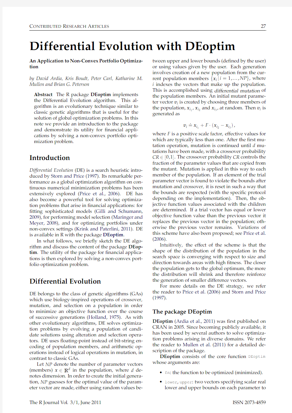
The global minimum is zero at point x=(0,0) .A
Figure1:Perspective plot of the Rastrigin function.
The function DEoptim searches for a minimum of the objective function between lower and upper bounds.A call to DEoptim can be made as follows:>set.seed(1234)
>DEoptim(fn=Rastrigin,
+lower=c(-5,-5),
+upper=c(5,5),
+control=list(storepopfrom=1))
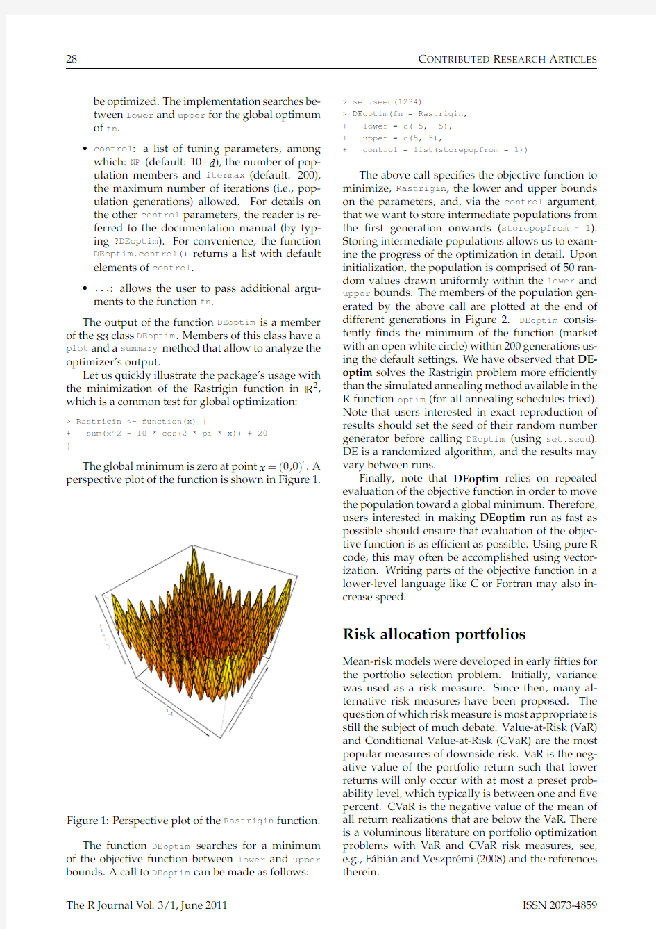
The above call speci?es the objective function to minimize,Rastrigin,the lower and upper bounds on the parameters,and,via the control argument, that we want to store intermediate populations from the?rst generation onwards(storepopfrom=1). Storing intermediate populations allows us to exam-ine the progress of the optimization in detail.Upon initialization,the population is comprised of50ran-dom values drawn uniformly within the lower and upper bounds.The members of the population gen-erated by the above call are plotted at the end of different generations in Figure2.DEoptim consis-tently?nds the minimum of the function(market with an open white circle)within200generations us-ing the default settings.We have observed that DE-optim solves the Rastrigin problem more ef?ciently than the simulated annealing method available in the R function optim(for all annealing schedules tried). Note that users interested in exact reproduction of results should set the seed of their random number generator before calling DEoptim(using set.seed). DE is a randomized algorithm,and the results may vary between runs.
Finally,note that DEoptim relies on repeated evaluation of the objective function in order to move the population toward a global minimum.Therefore, users interested in making DEoptim run as fast as possible should ensure that evaluation of the objec-tive function is as ef?cient as https://www.doczj.com/doc/686010082.html,ing pure R code,this may often be accomplished using vector-ization.Writing parts of the objective function in a lower-level language like C or Fortran may also in-crease speed.
Risk allocation portfolios
Mean-risk models were developed in early?fties for the portfolio selection problem.Initially,variance was used as a risk measure.Since then,many al-ternative risk measures have been proposed.The question of which risk measure is most appropriate is still the subject of much debate.Value-at-Risk(VaR) and Conditional Value-at-Risk(CVaR)are the most popular measures of downside risk.VaR is the neg-ative value of the portfolio return such that lower returns will only occur with at most a preset prob-ability level,which typically is between one and?ve percent.CVaR is the negative value of the mean of all return realizations that are below the VaR.There is a voluminous literature on portfolio optimization problems with VaR and CVaR risk measures,see, e.g.,Fábián and Veszprémi(2008)and the references therein.
Generation 1x 1
x 2
?4
?2024?4?2
02
4
Generation 20
x 1
x 2
?4
?2024?4?2
02
4
Generation 40x 1
x 2
?4
?2024?4?2
02
4
Generation 80
x 1
x 2
?4
?2024?4?2
02
4
Figure 2:The population (market with black dots)associated with various generations of a call to DEoptim as it searches for the minimum of the Rastrigin function at point x =(0,0) (market with an open white circle).The minimum is consistently determined within 200generations using the default settings of DEoptim .
Modern portfolio selection considers additional criteria such as to maximize upper-tail skewness and liquidity or minimize the number of securities in the portfolio.In the recent portfolio literature,it has been advocated by various authors to incorporate risk contributions in the portfolio allocation prob-lem.Qian’s (2005)Risk Parity Portfolio allocates port-folio variance equally across the portfolio compo-nents.Maillard et al.(2010)call this the Equally-Weighted Risk Contribution (ERC)Portfolio .They de-rive the theoretical properties of the ERC portfolio and show that its volatility is located between those of the minimum variance and equal-weight portfo-lio.Zhu et al.(2010)study optimal mean-variance portfolio selection under a direct constraint on the contributions to portfolio variance.Because the re-sulting optimization model is a non-convex quadrat-ically constrained quadratic programming problem,they develop a branch-and-bound algorithm to solve it.
Boudt et al.(2010a )propose to use the contribu-tions to portfolio CVaR as an input in the portfolio optimization problem to create portfolios whose per-centage CVaR contributions are aligned with the de-sired level of CVaR risk diversi?cation.Under the assumption of normality,the percentage CVaR con-tribution of asset i is given by the following explicit
function of the vector of weights w .
=(w 1,...,w d ) ,
mean vector μ.
=(μ1,...,μd ) and covariance matrix Σ:
w i
?μi +(Σw )i √w
Σw φ(z α)
α
?w μ+√w Σw φ(z α)α,with z αthe α-quantile of the standard normal distri-bution and φ(·)the standard normal density func-tion.Throughout the paper we set α=5%.As we
show here,the package DEoptim is well suited to solve these problems.Note that it is also the evo-lutionary optimization strategy used in the package PortfolioAnalytics (Boudt et al.,2010b ).
To illustrate this,consider as a stylized example a ?ve-asset portfolio invested in the stocks with tickers GE,IBM,JPM,MSFT and WMT.We keep the dimen-sion of the problem low in order to allow interested users to reproduce the results using a personal com-puter.More realistic portfolio applications can be obtained in a straightforward manner from the code below,by expanding the number of parameters opti-mized.Interested readers can also see the DEoptim package vignette for a 100-parameter portfolio opti-mization problem that is typical of those encountered in practice.
We ?rst download ten years of monthly data us-ing the function getSymbols of the package quant-mod (Ryan ,2010).Then we compute the log-return series and the mean and covariance matrix estima-tors.For on overview of alternative estimators of the covariance matrix,such as outlier robust or shrink-age estimators,and their implementation in portfolio allocation,we refer the reader to Würtz et al.(2009,Chapter 4).These estimators might yield better per-formance in the case of small samples,outliers or de-partures from normality.
>library("quantmod")
>tickers <-c("GE","IBM","JPM","MSFT","WMT")>getSymbols(tickers,+from ="2000-12-01",+to ="2010-12-31")>P <-NULL
>for(ticker in tickers){
+tmp <-Cl(to.monthly(eval(parse(text =ticker))))+P <-cbind(P,tmp)+}
>colnames(P)<-tickers >R <-diff(log(P))>R <-R[-1,]
>mu <-colMeans(R)>
sigma <-cov(R)
We ?rst compute the equal-weight portfolio.This is the portfolio with the highest weight diversi?ca-tion and often used as a benchmark.But is the risk exposure of this portfolio effectively well diversi?ed across the different assets?This question can be an-swered by computing the percentage CVaR contribu-tions with function ES in the package Performance-Analytics (Carl and Peterson ,2011).These percent-age CVaR contributions indicate how much each as-set contributes to the total portfolio CVaR.
>library("PerformanceAnalytics")
>pContribCVaR <-ES(weights =rep(0.2,5),+method ="gaussian",+portfolio_method ="component",+mu =mu,+sigma =sigma)$pct_contrib_ES
>rbind(tickers,round(100*pContribCVaR,2))
[,1][,2][,3][,4][,5]
tickers "GE""IBM""JPM""MSFT""WMT"
"21.61""18.6""25.1""25.39""9.3"
We see that in the equal-weight portfolio,25.39%of the portfolio CVaR risk is caused by the 20%investment in MSFT,while the 20%investment in WMT only causes 9.3%of total portfolio CVaR.The high risk contribution of MSFT is due to its high stan-dard deviation and low average return (reported in percent):
>round(100
*mu ,2)GE IBM JPM MSFT WMT -0.800.46-0.06-0.370.0
>round(100
*diag(sigma)^(1/2),2)GE IBM JPM MSFT WMT 8.907.95
9.6510.47 5.33
We now use the function DEoptim of the package DEoptim to ?nd the portfolio weights for which the portfolio has the lowest CVaR and each investment can contribute at most 22.5%to total portfolio CVaR
risk.For this,we?rst de?ne our objective function to minimize.The current implementation of DEop-tim allows for constraints on the domain space.To include the risk budget constraints,we add them to the objective function through a penalty function.As such,we allow the search algorithm to consider in-feasible solutions.A portfolio which is unacceptable for the investor must be penalized enough to be re-jected by the minimization process and the larger the violation of the constraint,the larger the increase in the value of the objective function.A standard ex-pression of these violations isα×|violation|p.Crama and Schyns(2003)describe several ways to calibrate the scaling factorsαand p.If these values are too small,then the penalties do not play their expected role and the?nal solution may be infeasible.On the other hand,ifαand p are too large,then the CVaR term becomes negligible with respect to the penalty; thus,small variations of w can lead to large varia-tions of the penalty term,which mask the effect on the portfolio CVaR.We setα=103and p=1,but recognize that better choices may be possible and de-pend on the problem at hand.
>obj<-function(w){
+if(sum(w)==0){w<-w+1e-2}
+w<-w/sum(w)
+CVaR<-ES(weights=w,
+method="gaussian",
+portfolio_method="component",
+mu=mu,
+sigma=sigma)
+tmp1<-CVaR$ES
+tmp2<-max(CVaR$pct_contrib_ES-0.225,0)
+out<-tmp1+1e3*tmp2
+}
The penalty introduced in the objective func-tion is non-differentiable and therefore standard gradient-based optimization routines cannot be used.In contrast,DEoptim is designed to consistently ?nd a good approximation to the global minimum of the optimization problem:
>set.seed(1234)
>out<-DEoptim(fn=obj,
+lower=rep(0,5),
+upper=rep(1,5))
>out$optim$bestval
[1]0.1143538
>wstar<-out$optim$bestmem
>wstar<-wstar/sum(wstar)
>rbind(tickers,round(100*wstar,2))
par1par2par3par4par5 tickers"GE""IBM""JPM""MSFT""WMT"
"18.53""21.19""11.61""13.37""35.3"
>100*(sum(wstar*mu)-mean(mu))
[1]0.04827935
Note that the main differences with the equal-weight portfolio is the low weights given to JPM and MSFT and the high weight to WMT.As can be seen from the last two lines,this minimum risk portfolio has a higher expected return than the equal weight portfolio.The following code illustrates that DEop-tim yields superior results than the gradient-based optimization routines available in R.
>out<-optim(par=rep(0.2,5),
+fn=obj,
+method="L-BFGS-B",
+lower=rep(0,5),
+upper=rep(1,5))
>out$value
[1]0.1255093
>out<-nlminb(start=rep(0.2,5),
+objective=obj,
+lower=rep(0,5),
+upper=rep(1,5))
>out$objective
[1]0.1158250
Even on this relatively simple stylized example, the optim and nlminb routines converged to local minima.
Suppose now the investor is interested in the most risk diversi?ed portfolio whose expected re-turn is higher than the equal-weight portfolio.This amounts to minimizing the largest CVaR contribu-tion subject to a return target and can be imple-mented as follows:
>obj<-function(w){
+if(sum(w)==0){w<-w+1e-2}
+w<-w/sum(w)
+contribCVaR<-ES(weights=w,
+method="gaussian",
+portfolio_method="component",
+mu=mu,
+sigma=sigma)$contribution
+tmp1<-max(contribCVaR)
+tmp2<-max(mean(mu)-sum(w*mu),0)
+out<-tmp1+1e3*tmp2
+}
>set.seed(1234)
>out<-DEoptim(fn=obj,
+lower=rep(0,5),
+upper=rep(1,5))
>wstar<-out$optim$bestmem
>wstar<-wstar/sum(wstar)
>rbind(tickers,round(100*wstar,2))
par1par2par3par4par5 tickers"GE""IBM""JPM""MSFT""WMT"
"17.38""19.61""14.85""15.19""32.98"
>100*(sum(wstar*mu)-mean(mu))
[1]0.04150506
This portfolio invests more in the JPM stock and less in the GE(which has the lowest average return) compared to the portfolio with the upper22.5%per-centage CVaR constraint.We refer to Boudt et al. (2010a)for a more elaborate study on using CVaR al-locations as an objective function or constraint in the portfolio optimization problem.
A classic risk/return(i.e.,CVaR/mean)scatter chart showing the results for portfolios tested by
DEoptim is displayed in Figure3.Gray elements depict the results for all tested portfolios(using hexagon binning which is a form of bivariate his-togram,see Carr et al.(2011);higher density regions are darker).The yellow-red line shows the path of the best member of the population over time,with the darkest solution at the end being the optimal port-folio.We can notice how DEoptim does not spend much time computing solutions in the scatter space that are suboptimal,but concentrates the bulk of the calculation time in the vicinity of the?nal best port-folio.Note that we are not looking for the tangency portfolio;simple mean/CVaR optimization can be achieved with standard optimizers.We are looking here for the best balance between return and risk con-centration.
We have utilized the mean return/CVaR concen-tration examples here as more realistic,but still styl-ized,examples of non-convex objectives and con-straints in portfolio optimization;other non-convex objectives,such as drawdown minimization,are also common in real portfolios,and are likewise suitable to application of Differential Evolution.One of the key issues in practice with real portfolios is that a portfolio manager rarely has only a single objective or only a few simple objectives combined.For many combinations of objectives,there is no unique global optimum,and the constraints and objectives formed lead to a non-convex search space.It may take sev-eral hours on very fast machines to get the best an-swers,and the best answers may not be a true global optimum,they are just as close as feasible given poten-tially competing and contradictory objectives.
When the constraints and objectives are relatively simple,and may be reduced to quadratic,linear,or conical forms,a simpler optimization solver will pro-duce answers more quickly.When the objectives are more layered,complex,and potentially contra-dictory,as those in real portfolios tend to be,DE-optim or other global optimization algorithms such as those integrated into PortfolioAnalytics provide a portfolio manager with a feasible option for opti-mizing their portfolio under real-world non-convex constraints and objectives.
The PortfolioAnalytics framework allows any ar-bitrary R function to be part of the objective set,and allows the user to set the relative weighting that they want on any speci?c objective,and use the appropri-ately tuned optimization solver algorithm to locate portfolios that most closely match those objectives. Summary
In this note we have introduced DE and DEoptim. The package DEoptim provides a means of applying the DE algorithm in the R language and environment for statistical computing.DE and the package DE-optim have proven themselves to be powerful tools for the solution of global optimization problems in a wide variety of?elds.We have referred interested users to Price et al.(2006)and Mullen et al.(2011)for a more extensive introduction,and further pointers to the literature on DE.The utility of using DEoptim was further demonstrated with a simple example of a stylized non-convex portfolio risk contribution allo-cation,with users referred to PortfolioAnalytics for portfolio optimization using DE with real portfolios under non-convex constraints and objectives.
The latest version of the package includes the adaptive Differential Evolution framework by Zhang and Sanderson(2009).Future work will also be di-rected at parallelization of the implementation.The DEoptim project is hosted on R-forge at https:// https://www.doczj.com/doc/686010082.html,/projects/deoptim/. Acknowledgements
The authors would like to thank Dirk Eddelbuettel, Juan Ospina,and Enrico Schumann for useful com-ments and Rainer Storn for his advocacy of DE and making his code publicly available.The authors are also grateful to two anonymous reviewers for help-ful comments that have led to improvements of this note.Kris Boudt gratefully acknowledges?nancial support from the National Bank of Belgium. Disclaimer
The views expressed in this note are the sole respon-sibility of the authors and do not necessarily re?ect those of aeris CAPITAL AG,Guidance Capital Man-agement,Cheiron Trading,or any of their af?liates. Any remaining errors or shortcomings are the au-thors’responsibility.
Bibliography
D.Ardia,K.M.Mullen,B.G.Peterson and J.Ulrich. DEoptim:Differential Evolution Optimization in R, 2011.URL https://www.doczj.com/doc/686010082.html,/package= DEoptim.R package version2.1-0.
K.Boudt,P.Carl,and B.G.Peterson.Portfolio op-timization with conditional value-at-risk budgets. Working paper,2010a.
K.Boudt,P.Carl,and B.G.Peterson.Port-folioAnalytics:Portfolio Analysis,including Nu-meric Methods for Optimization of Portfolios,2010b. URL https://www.doczj.com/doc/686010082.html,/projects/ returnanalytics/.R package version0.6.
P.Carl and B.G.Peterson.PerformanceAnalytics: Econometric tools for performance and risk analy-sis.,2011.URL https://www.doczj.com/doc/686010082.html,/
141618202224
?0.4
?0.2
0.2
0.4
monthly CVaR (in %)
m o n t h l y m e a n (i n %
)
Figure 3:Risk/return scatter chart showing the results for portfolios tested by DEoptim .
projects/returnanalytics/.R package version
1.0.3.3.
D.Carr,N.Lewin-Koh and M.Maechler.hexbin: Hexagonal binning routines,2011.URL http:// https://www.doczj.com/doc/686010082.html,/package=hexbin.R package version1.26.0
Y.Crama and M.Schyns.Simulated annealing for complex portfolio selection problems.European Journal of Operations Research,150(3):546–571,2003.
C.Fábián and A.Veszprémi.Algorithms for han-dling CVaR constraints in dynamic stochastic pro-gramming models with applications to?nance. Journal of Risk,10(3):111–131,2008.
M.Gilli and E.Schumann.Heuristic optimisa-tion in?nancial https://www.doczj.com/doc/686010082.html,ISEF wps-007 09/02/2009,2009.
J.H.Holland.Adaptation in Natural Arti?cial Systems. University of Michigan Press,1975.
T.Krink and S.Paterlini.Multiobjective optimization using Differential Evolution for real-world portfo-lio https://www.doczj.com/doc/686010082.html,putational Management Sci-ence,8:157–179,2011.
S.Maillard,T.Roncalli,and J.Teiletche.On the prop-erties of equally-weighted risk contributions port-folios.Journal of Portfolio Management,36(4):60–70, 2010.
D.G.Maringer and M.Meyer.Smooth transition autoregressive models:New approaches to the model selection problem.Studies in Nonlinear Dy-namics&Econometrics,12(1):1–19,2008.
K.M.Mullen,D.Ardia,D.L.Gil,D.Windover,and J.Cline.DEoptim:An R package for global opti-mization by Differential Evolution.Journal of Sta-tistical Software,40(6):1–26,2011.
K.V.Price,R.M.Storn,and https://www.doczj.com/doc/686010082.html,mpinen.Differ-ential Evolution:A Practical Approach to Global Opti-mization.Springer-Verlag,Berlin,Heidelberg,sec-ond edition,2006.ISBN3540209506.
E.Qian.Risk parity portfolios:Ef?cient portfolios through true diversi?cation of risk.PanAgora As-set Management working paper,2005.J.A.Ryan.quantmod:Quantitative Financial Modelling Framework,2010.URL http://CRAN.R-project. org/package=quantmod.R package version0.3-16. O.Scaillet.Nonparametric estimation and sensitiv-ity analysis of expected shortfall.Mathematical Fi-nance,14(1):74–86,2002.
R.Storn and K.Price.Differential Evolution–A sim-ple and ef?cient heuristic for global optimization over continuous spaces.Journal of Global Optimiza-tion,11:341–359,1997.
D.Würtz,Y.Chalabi,W.Chen and A.Ellis Portfolio Optimization with R/Rmetrics.Rmetrics Association and Finance Online,2009.
J.Zhang and A. C.Sanderson.JADE:Adap-tive Differential Evolution with optional external archive.IEEE Transactions on Evolutionary Compu-tation,13(5):945–958,2009.
S.Zhu,D.Li,and X.Sun.Portfolio selection with marginal risk control.Journal of Computational Fi-nance,14(1):1–26,2010.
David Ardia
aeris CAPITAL AG,Switzerland
da@https://www.doczj.com/doc/686010082.html,
Kris Boudt
Lessius and K.U.Leuven,Belgium
kris.boudt@econ.kuleuven.be
Peter Carl
Guidance Capital Management,Chicago,IL
pcarl@https://www.doczj.com/doc/686010082.html,
Katharine M.Mullen
National Institute of Standards and Technology Gaithersburg,MD
katharine.mullen@https://www.doczj.com/doc/686010082.html,
Brian G.Peterson
Cheiron Trading,Chicago,IL
brian@https://www.doczj.com/doc/686010082.html,
南车四方机车车辆股份有限公司 青岛喜盈门集团公司 青岛广源发集团有限公司 青岛美高集团有限公司 济南山水集团有限公司青岛水泥分公司青岛正进集团有限公司 青岛大农服装有限公司 山东黄岛发电厂 青岛金晶股份有限公司 青岛恒源热电有限公司 青岛浮法玻璃有限公司 青岛压花玻璃有限公司 青岛市圣戈班韩洛玻玻璃有限公司 青岛高合有限公司 青岛浦项不锈钢有限公司 青岛北海船舶重工有限责任公司 青岛经济技术开发区热电燃气总公司 青岛赛轮子午线轮胎信息化生产示范基地 1 即墨市热电厂 青岛即发集团控股有限公司 青岛新源热电有限公司 青岛三湖制鞋有限公司 青岛正大有限公司 青岛高丽钢线有限公司 青岛北汇玻璃有限公司 即墨市双春水泥有限公司 青岛红领服饰股份有限公司 青岛恒光热电有限公司 青岛恒源化工有限公司 青岛天元化工股份有限公司 青岛海王纸业股份有限公司 青岛琅琊台酒业(集团)股份有限公司青岛胶南明月海藻工业有限责任公司 胶南易通热电有限责任公司 青岛泰发集团股份有限公司 青岛东亚轮胎有限公司
青岛康大外贸集团有限公司 胶南供电公司 胶南市水泥厂 2 胶南市海龙福利板纸有限公司 青岛振华工业集团有限公司 青岛德固萨化学有限公司 青岛龙发热电有限公司 青岛恒祥化肥有限公司 青岛世原鞋业有限公司 青岛华威建材有限公司 青岛广源发玻璃有限公司 青岛大明皮革有限公司 青岛昌新鞋业有限公司 青岛衣东纺织有限公司 青岛海尔金塑制品有限公司 山东金湖水泥有限公司青岛分公司 青岛福生食品有限公司 青岛信五皮革有限公司 青岛多福康食品有限公司 胶州天成玻璃工艺品厂 胶州市新纪元帘子布有限公司 青岛昌华集团股份有限公司 青岛热电集团金莱热电有限公司 青岛金浪热电有限公司 3 青岛泰光制鞋有限公司 青岛现代人热力发展有限公司 青岛金浪化工集团有限公司 青岛凤凰东翔印染有限公司 青岛九联集团股份有限公司 青岛海升果业有限责任公司 青岛交河技工塑料有限公司 青岛东方化工股份有限公司 海尔集团公司 青岛崂山玻璃有限公司 青岛啤酒第五有限公司
注意:以下内容请进一步总结! 青岛恒源热电有限公司 目标公司主要从事蒸汽、热水的生产及供应、蒸汽余热发电业务,同时提供供热管道及设施维修、安装业务。据介绍,目标公司开发了循环水供热工程项目,该项目是青岛市获批的第一个清洁发展机制(CDM)项目;前处该项目处于施工建设阶段,预计将于2009年上半年内正式投产。据介绍,目标公司主要负责临港工业区辖区内的蒸汽供应及热网管理,发电业务,对居民的用热服务。 公司成立于2001年,主要从事蒸汽、热水的生产及供应、蒸汽余热发电业务。 青岛恒源热电有限公司位于开发区B区供热范围,拥有12MW的抽凝式汽轮发电机组1台及12MW的背压机组1台,75t/h循环流化床锅炉3台和150t/h锅炉1台,最大供热能力是355t/h,担负着B区的生产、民用供热负荷,主要满足热电厂东部居民小区供热和山东科技大学供热。 青岛恒源热电有限公司位于青岛经济技术开发区临港工业区的中北部,海尔大道与渭河路交界处东北角,渭河路777号。厂区所在地东侧隔宽约100m绿化地为鑫龙物流公司,该公司东侧、距离本项目最近300m处为澳柯玛人才公寓;厂区南侧隔渭河路、绿化带100m处为东小庄村(原村庄平房已搬迁,现建有多座两层复式楼房),该村庄南侧、距离本项目约420m处为山孚日水食品有限公司;项目隔渭河路东南方向约200m处为澳柯玛工业园;西及西南方向隔海尔大道、渭河路均为浦项制铁有限公司;北侧与开发区消防大队以及正友砼业相邻。 企业所在地厂址东南距市中心约8km,东面距前湾港区约4.5km。 现有工程内容:青岛恒源热电有限公司主要服务于黄岛供热分区B 区(齐长城路以北、疏港高速以南、镰湾河以西、柳花泊和珠山以东片区(包括柳花泊),总占地面积约60平方公里)。企业现有锅炉规模为3×75t/h+1×130t/h 循环流化床蒸汽锅炉,总计约355t/h锅炉容量;发电机组规模为1×12MW C12-34.9/0.98(抽凝)+1×12MW B12-4.9/0.98(背压),总计发电装机容量24 MW。 近几年,恒源热电强化能源管理,合理调整运行方式,加强节能技术改造,企业能源管理工作上了一个新台阶,先后通过了“企业能源审计”、“热电联产机组认定”等审核认证工作,被评为“青岛市清洁生产企业”,2007年度“山东省节能先进企业”。 为进一步加强企业能源管理,完善优化企业节能减排工作,公司在本年度开始推行循环经济试点工作。目前,作为试点工作重点项目之一的企业冷渣机改造项目已基本完成,初步具备投运条件,预计本年度六月份正式投入运行。该项目是将循环流化床锅炉的人工排渣(温度一般在900℃),通过加装冷渣机把炉渣余热加热除盐水,将锅炉效率提高1-3%,同时解决人工放渣存在安全隐患、能源浪费以及不环保等问题,项目投资为85万元,年可节标煤700吨。
热能与动力工程专业制热方向认识 实习报告 学院:机电工程学院 班级:热能一班 姓名:徐国庆 学号:201240502013
一.认识实习的目的和任务 1.认识实习的目的: (1)认识实习是四年制高等学校教学活动的实践环节之一; (2)认识实习是对学生进行火力发电厂主机(锅炉、汽轮机)、辅机(换热器、风机、水泵)及其制造厂的设备系统、生产工艺进行认识性训 练,对发电厂热力系统进行整体初步了解。 2.认识实习的任务: (1)对火力发电厂主机的认识实习 实习对象:锅炉本体、汽轮发电机本体。锅炉形式包括煤粉锅炉、循 环流化床锅炉、链条炉、余热锅炉等。汽轮机形式包括凝气式汽轮机、 背压式汽轮机、调节抽汽式汽轮机。 认识内容:设备外形特点、摆放位置、主要性能参数、安全生产常识。 (2)对火力发电厂辅助机械设备的认识实习 实习对象:制粉系统、除尘除灰系统、烟风系统、回热系统、润滑冷 却系统、水油净化系统等。 认识内容:设备外形特点、摆放位置、主要性能参数、安全生产常识。 (3)对火力发电厂设备系统的认识实习 实习对象:火力发电厂主机和辅机工程的系统。 认识内容:设备之间的空间关系、安全生产常识。 3.认识实习的意义 (1)强化学生对专业基础课程的理解 (2)国内火力发电厂的技术发展出现了新进展 CFB锅炉、燃气轮机、余热锅炉、超临界机组、烟气脱硫、布袋除尘、集中控制运行等新技术。 (3)认识实习有利于培养学生的职业精神 (4)认识实习有利于了解机组 (5)认识实习有利于了解机组建设过程 二.捷能汽轮机厂 (1)简介:汽轮机是火力发电厂三大主要设备之一。它是以蒸汽为工质,将热能转变为机械能的高速旋转式原动机。它为发电机的能量转换提供机 械能。 青岛捷能汽轮机集团股份有限公司始建于1950年,是我国汽轮机行业重 点骨干企业。拥有各种数控、数显等机械加工设备2200余台,以200MW 及以下“捷能牌”汽轮机为主导产品,拥有电站汽轮机和工业拖动汽轮 机两大系列产品,能够满足发电、石化、水泥、冶金、造纸、垃圾处理、燃气-蒸汽联合循环、城市集中供热等领域需求,年产能达500台/600万 千瓦以上。中小型汽轮机市场占有率居国内同行业首位,是目前国内中 小型汽轮机最大最强的设计制造供应商和电站成套工程总包商。 公司积极推进品牌战略,率先在汽轮机行业内取得了美国FMRC公司双重 ISO9001国际质量体系认证和ISO1400环境管理体系认证,率先在汽轮机 行业内第一个获得了“中国名牌产品”称号,先后获得了“全国AAA级 信用企业”、“中国优秀诚信企业”、“全国用户满意产品”、“山东
供热管网检修作业指导手册[青岛热电集团] 供热管网检修作业指导手册[青岛热电集团] 供热管网检修作业指导手册[青岛热电集团] 作者:佚名更新时间:2008-12-5 15:55:38 字体: 供热管网检修作业指导手册 1 总则 1.1 为使公司供热管网的维护、检修工作更为规范和科学合理,确保安全运行,制定作业指导手册。 1.2 本作业指导手册适用于公司供热管网的维护、检修及事故抢修。 本作业指导手册供热管网的工作压力限定为: 工作压力不大于1.6MPa(表压),介质温度不大于300?的蒸汽供热管网。 1.3 管网的检修工作应符合原设计要求。 1.4 执行本作业指导手册时,尚应符合国家现行有关标准的规定。 2 术语 2.1 热网维修 热网的维护和检修。本作业指导手册中简称维修。 2.2 热网维护 供热运行期间,在不停热条件下对热网进行的维护工作。本作业指导手册中简称维护。 2.3 热网检修 在停热条件下对热网进行的检修工作。本作业指导手册中简称检修。 2.4 热网抢修
供热管道设备突发故障引起蒸汽大量泄漏,危及管网安全运行或对周边环境、人身安全造成威胁时进行的紧急检修工作。本作业指导手册中简称抢修。 2.5 供热管网 由热源向热用户输送和分配供热介质的管线系统。本作业指导手册中简称热网。 3 维护、检修机构设置、检修人员及设备 3.1 维护、检修机构设置及人员要求 3.1.1客户服务中心是公司高新区内供热管网运行、调度、维护、检修的责任机构,负责高新区内供热管网的维护、检修工作。 3.1.2 供热管冈的维护、检修人员必须经过培训和专业资格考 试合格后,方可独立进行维护、检修工作。供热管网维护、检修人员必须熟悉管辖范围内的管道分布情况、设备及附件位置。维护、检修人员必须掌握管辖范国内供热管线各种附件的作用、性能、构造以及安装操作和维护、检修方法。 3.1.3检修人员出门检修时应穿公司工作服,配戴上岗证,注意礼貌用语,维护公司形象。 3.2 维护、检修用主要设备与器材 3.2.1 供热管网的维护检修部门,应备有维护、检修及故障抢修时常用的设备与器材。 3.2.2检修设备、工具平时摆放在规定位置,检修设备和专用工具要有专人保管,所有设备、工具应保证完好,须保证检修时能够立即投入使用。检修物资也应分门别类码放整齐,方便查找,以保证检修、抢修时不会因为寻找物资配件而耽误时间。每次检修完后都应检查备品备件数量,发现不够时要及时与物质采购部联系进行必要地补充,确保检修时不会因无备品备件而影响检修时间与质量。
招标投标企业报告 青岛西海岸公用事业集团易通热电有限公司新 能源分公司
本报告于 2019年9月22日 生成 您所看到的报告内容为截至该时间点该公司的数据快照 目录 1. 基本信息:工商信息 2. 招投标情况:中标/投标数量、中标/投标情况、中标/投标行业分布、参与投标 的甲方排名、合作甲方排名 3. 股东及出资信息 4. 风险信息:经营异常、股权出资、动产抵押、税务信息、行政处罚 5. 企业信息:工程人员、企业资质 * 敬启者:本报告内容是中国比地招标网接收您的委托,查询公开信息所得结果。中国比地招标网不对该查询结果的全面、准确、真实性负责。本报告应仅为您的决策提供参考。
一、基本信息 1. 工商信息 企业名称:青岛西海岸公用事业集团易通热电有限公司新能 源分公司 统一社会信用代码:91370211334195493K 工商注册号:370211120004502组织机构代码:334195493法定代表人:赵军田成立日期:2015-04-23 企业类型:有限责任公司分公司(非自然人投资或控股的法人 独资) 经营状态:注销 注册资本:/ 注册地址:山东省青岛市黄岛区相公山路723号 营业期限:2015-04-23 至 / 营业范围:为上级公司联系业务。(依法须经批准的项目,经相关部门批准后方可开展经营活动)联系电话:*********** 二、招投标分析 2.1 中标/投标数量 企业中标/投标数: 个 (数据统计时间:2017年至报告生成时间)
2.2 中标/投标情况(近一年) 截止2019年9月22日,根据国内相关网站检索以及中国比地招标网数据库分析,未查询到相关信息。不排除因信息公开来源尚未公开、公开形式存在差异等情况导致的信息与客观事实不完全一致的情形。仅供客户参考。 2.3 中标/投标行业分布(近一年) 截止2019年9月22日,根据国内相关网站检索以及中国比地招标网数据库分析,未查询到相关信息。不排除因信息公开来源尚未公开、公开形式存在差异等情况导致的信息与客观事实不完全一致的情形。仅供客户参考。 2.4 参与投标的甲方前五名(近一年) 截止2019年9月22日,根据国内相关网站检索以及中国比地招标网数据库分析,未查询到相关信息。不排除因信息公开来源尚未公开、公开形式存在差异等情况导致的信息与客观事实不完全一致的情形。仅供客户参考。 2.5 合作甲方前五名(近一年) 截止2019年9月22日,根据国内相关网站检索以及中国比地招标网数据库分析,未查询到相关信息。不排除因信息公开来源尚未公开、公开形式存在差异等情况导致的信息与客观事实不完全一致的情形。仅供客户参考。 三、股东及出资信息 截止2019年9月22日,根据国内相关网站检索以及中国比地招标网数据库分析,未查询到相关信息。不排除因信息公开来源尚未公开、公开形式存在差异等情况导致的信息与客观事实不完全一致的情形。仅供客户参考。 四、风险信息 4.1 经营异常() 截止2019年9月22日,根据国内相关网站检索以及中国比地招标网数据库分析,未查询到相关信息。不排除因信息公开来源尚未公开、公开形式存在差异等情况导致的信息与客观事实不完全一致的情形。仅供客户参考。 4.2 股权出资() 截止2019年9月22日,根据国内相关网站检索以及中国比地招标网数据库分析,未查询到相关信息。不排除因信息公开来源尚未公开、公开形式存在差异等情况导致的信息与客观事实不完全一致的情形。仅供客户参考。 4.3 动产抵押() 截止2019年9月22日,根据国内相关网站检索以及中国比地招标网数据库分析,未查询到相关信息。不排除因信息公开来源尚未公开、公开形式存在差异等情况导致的信息与客观事实不完全一致的情形。仅供客户参考。 4.4 税务信息() 截止2019年9月22日,根据国内相关网站检索以及中国比地招标网数据库分析,未查询到相关信息。不排除因信息公开来源尚未公开、公开形式存在差异等情况导致的信息与客观事实不完全一致的情形。仅供客户参考。
青岛热电集团有限公司成立于1993年,属于国有独资大型热电联产企业,主要担负着青岛市企、事业单位和居民供热及部分发电任务,同时,供热市场辐射黄岛、平度、莱西、即墨、城阳等县市区域。集团公司先后成立了工程公司和具有甲级设计资质的设计院,逐步形成了热电联产、区域锅炉、热网输配等多种供热形式并存,集供热、发电、热力设计、工程施工、热力产品制造经营为一体的完整产业链。 目前,热电集团为全省地方最大供热企业。企业资产总额48亿元,年销售收入16.2亿元,所属企业16个,职工2200余人,年供蒸汽312万吨,年发电能力9.3万千瓦,已建成蒸汽管网145.43公里,热水管网1552.93公里,供(换)热站294座,供热面积3561万平方米,拥有单位用户292家,居民用户28.8万余户。 集团公司先后被评为全国AAA级信用企业、全国建设系统文明服务示范窗口单位、思想政治工作先进单位、企业文化建设先进单位、精神文明建设先进单位;山东省文明单位、节能先进企业、思想政治工作优秀企业;青岛市和工商年度免检企业、安全生产先进单位、廉洁勤政先进单位;山东省供热协会副理事长单位。 自成立以来,公司始终秉承“关爱社会、服务民生”的企业宗旨和“励精图治、锲而不舍”的企业精神,贯彻科学发展,创新经营管理,实现了企业快速发展。1996年在全国供热行业首家推出社会服务责任赔偿制度,1997年在山东省供热行业首家进行了股份制改造,1998年在山东省供热行业首家成功地进行了集团产权制度改革,1999年在全国同行业中首家通过了ISO9001国际质量认证,并先后通过了ISO14001环境管理体系和GB/T28001-2001职业健康安全管理体系认证,2001年公司成为全国供热行业中首家申请注册服务商标的企业,推出“暖到家”服务品牌,并被评为山东省著名商标和服务名牌。“青岛热电”正在逐步步入标准化、规范化、品牌化的发展轨道。 招聘专业及人数: 1、结构专业1人(研究生); 2、建筑专业1人(研究生); 3、技经专业1人(研究生); 4、焊接技术与工程1人; 5、无损检测专业1人;
华能集团所属电厂: 华能丹东电厂华能大连电厂华能上安电厂华能德州电厂华能威海电厂华能济宁电厂华能日照电厂华能太仓电厂华能淮阴电厂华能南京电厂华能南通电厂华能上海石洞口第一电厂华能上海石洞口第二电厂华能长兴电厂华能福州电厂华能汕头燃煤电厂华能汕头燃机电厂华能玉环电厂华能沁北电厂华能榆社电厂华能辛店电厂华能重庆分公司华能井冈山电厂华能平凉电厂华能岳阳电厂华能营口电厂华能邯峰电厂 大唐集团所属: 长山热电厂湖南省石门电厂鸡西发电厂洛阳首阳山电厂洛阳热电厂三门峡华阳发电公司河北马头电力公司唐山发电总厂北京大唐张家口发电总厂兰州西固热电有限公司合肥二电厂田家庵发电厂北京大唐高井发电厂永昌电厂北京大唐陡河电厂南京下关发电厂安徽淮南洛河发电厂保定热电厂略阳发电厂微水发电厂峰峰发电厂含岳城电站天津大唐盘山发电公司内蒙大唐托克托发电公司保定余热电厂华源热电有限责任公司阳城国际发电有限公司辽源热电有限责任公司四平发电运营中心长春第二热电有限公司晖春发电有限责任公司鸡西热电有限责任公司佳木斯第二发电厂台河第一电厂江苏徐塘发电有限公司安徽省淮北发电厂安徽淮南洛能发电公司安阳华祥电力有限公司许昌龙岗发电有限公司华银电力株洲发电厂华银株洲发电公司金竹山电厂华银金竹山火力发电厂湘潭发电有限责任公司湖南省耒阳发电厂灞桥热电有限责任公司灞桥热电厂陕西渭河发电厂陕西延安发电厂陕西韩城发电厂永昌发电厂甘肃甘谷发电厂甘肃八0三发电厂甘肃连城发电厂甘肃兰西热电有限公司广西桂冠电力股份公司桂冠大化水力发电总厂广西岩滩水电厂陈村水力发电厂王快水电厂张家界水电开发公司贺龙水电厂鱼潭水电厂陕西石泉水力发电厂石泉发电有限责任公司甘肃碧口水电厂百龙滩电厂华电所属: 1中国华电工程(集团)有限公司2华电煤业集团有限公司3华电财务有限公司4华电招标有限公司5华信保险经纪有限公司6北京华信保险公估有限公司7河北热电有限责任公司8包头东华热电有限公司(在建)9内蒙古华电乌达热电有限公司(在建)10华电国际电力股份有限公司11华电国际电力股份有限公司邹县发电厂(扩建)12华电国际电力股份有限公司莱城发电厂13华电国际电力
青热电〔2010〕121号 青岛热电集团有限公司 关于实施供热计量收费工作的意见 各单位、处室: 为全面贯彻《山东省物价局、山东省住房和城乡建设厅关于推进供热计量改革的指导意见》,根据青热办【2010】25号文件要求,自2010年开始,新供热建筑及完成供热计量改造的既有居住建筑,取消以面积计价收费,实行按用热量计价收费,为做好供热计量收费工作,经研究确定以下实施意见: 一、实施计划 (一)对已经改造完成的既有居住建筑实施供热计量收费,明细如下:第一热力海信慧谷、丰华园、弘信花园、都市名家小区;第二热力公司天宝苑小区;金河热力公司荣馨苑小区。
(二)对新竣工非居住建筑全面按用热量计量收费。 二、实施措施: (一)加强组织领导,责任到位。 职责明确,责任到人。集团成立以董事长为组长,总经理为副组长的供热计量工作领导小组,工程开发处、生安处、财务处、服务处各司其职,全力做好供热计量收费实施工作。各所属生产单位必须成立工作领导小组,将宣传、收费、数据公示、政策答疑等工作落实到位,各单位要有专门的供热计量工作负责人。 (二)措施到位,计划周密。 责任部门要全力做好实施热计量收费工作的计划安排,配合相关科室做好用户协调、宣传、合同签订、数据公示以及收、退费工作。 (三)做好新建、竣工项目供热计量设施的管理工作。各相关部门要严格新建、在建、新竣工项目供热计量设施的审核、把关、验收和问题汇总工作。 三、工作要求 (一)做好用户宣传、解释工作。在张贴用户通知进行宣传的同时,相关人员要明确供热计量工作实施相关要求规定,收费方式以及供热调节方式等,做好对用户的宣传解释工作,让用户明白调节方式和收退费方式、时间等。 (二)做好用户结算工作。用户的供热计量数据要真实、准确,各单位要认真做好用户仪表底数(正式供热时间和停止供热时间)确认工作,并定时张贴通知公开热量数据。 (三)做好数据分析和总结。对供热数据按周期进行定
1建设项目概况 1.1建设项目背景及建设地点 1.1.1建设项目背景 青岛钢铁有限公司(以下简称青钢)始建于1958年,位于青岛市北李沧区,属城市钢铁厂。厂区东邻重庆路、南渠村;西围墙距胶济铁路约85m;北距流亭国际机场约3.8km;南靠遵义路。距市中心约15km,厂内铁路专线与胶济铁路娄山站接轨,全厂总占地面积不足1.3km2。 青钢是集焦化、烧结、炼铁、炼钢、轧钢、发电等为一体的钢铁联合企业,是山东省重要的优质棒线材生产基地,山东省三大钢铁支柱企业。 目前,青钢已形成年产铁、钢、材各400×104t的生产能力。其主要生产设施有:60×104t焦化厂;2×50m2烧结机,2×105m2烧结机;5×500+1×625m3高炉;一炼钢有4×35t转炉,5座30tLF精炼炉,3台4机4流R5m小方坯连铸机和1台4机4流R8m连铸机;二炼钢有2×80t 顶底复吹转炉,3座90tLF精炼炉,1座90tRH精炼炉,2台6机6流R9m 连铸机;轧钢车间有1#、2#、3#高速线材车间,复二重线材车间,半连续小型车间,横列式小型车间,还有与之配套的相应公辅设施。 青钢产品有:热轧盘条,热轧带肋钢筋、圆钢、扁钢等型钢。主要品种有:焊接用钢盘条、汽车用弹簧扁钢、硬线盘条、冷镦钢、PC钢棒用线材、拉丝线材、易切削钢、优质碳素结构圆钢、建筑用线材与螺纹钢等。2011年,青钢生产生铁330.69×10⁴t、钢318.27×10⁴t、钢材301.99×10⁴t。2011年工业总产值297.79亿元,工业销售产值299.47亿元。青钢现有产品以优特钢为主,品种结构具有特色,产品附加值高。青钢现有职工1万余人,其中各类工程技术人员约1500余人。 自1997年以来,青钢经过不断的技术改造,其生产能力和经济效益均有了较大幅度的提高,但由于历史原因,还存在许多问题,如产品结构性矛盾仍