
Make a simple worksheet and chart
Which country are the most students in the class from? Which country are the fewest from? You will survey the class about their home countries and then create a worksheet and chart showing the results.
I. Get your information
With the whole class, count how
many people are from which
countries. Someone will write the
information on the board. Copy the
information in your notebook.
II. Enter the information in
Excel
1.Start Microsoft Excel.
2.Click in cell A1.
3.Type Where are my classmates
from? Press the down arrow.
4.Type Country. Press the down
arrow.
5.Type the names of the
countries. Press the down arrow after each country.
6.Type Total.
7.Click in cell B2.
8.Type Number of students. Press the down arrow.
9.Type the numbers for each country. Press the down arrow after each number.
III. Calculate the total number of students
1.Click in the cell below the last number you typed.
2.Click the AutoSum button on the Standard Toolbar two times.
AutoSum button
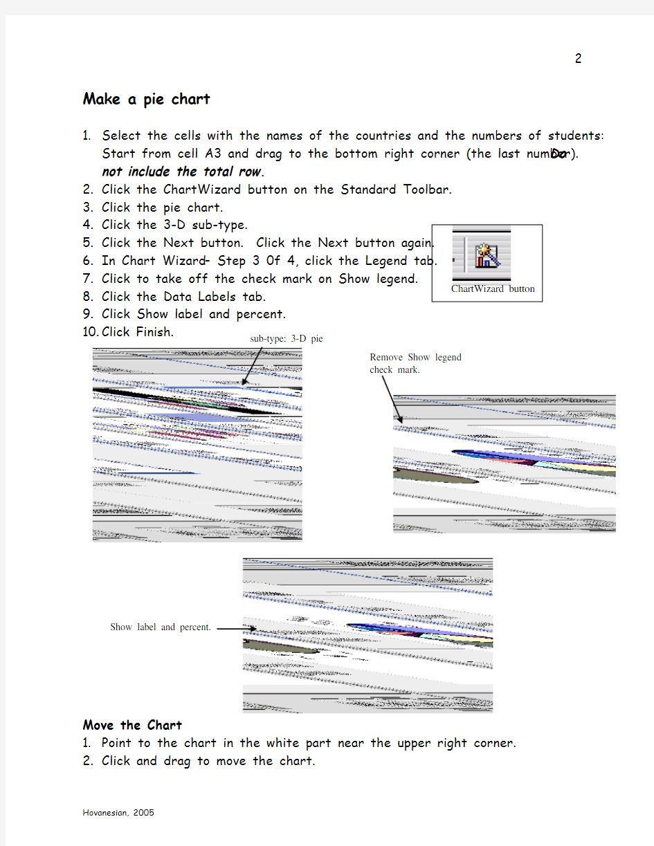
sub-type: 3-D pie Remove Show legend check mark. Show label and percent. Make a pie chart
1. Select the cells with the names of the countries and the numbers of students: Start from cell A3 and drag to the bottom right corner (the last number). Do not include the total row.
2. Click the ChartWizard button on the Standard Toolbar.
3. Click the pie chart.
4. Click the 3-D sub-type.
5. Click the Next button. Click the Next button again.
6. In Chart Wizard – Step 3 0f 4, click the Legend tab.
7. Click to take off the check mark on Show legend. 8. Click the Data Labels tab. 9. Click Show label and percent.
10. Click Finish.
Move the Chart
1. Point to the chart in the white part near the upper right corner.
2. Click and drag to move the chart.
ChartWizard button
Format the worksheet:Use the Formatting toolbar
A. Format the title
1.Click in cell A1. Change the Font Size to 14.
2.Click the Font Color button. Change the color (you choose it).
3.Click the Font button. Change the font (you choose it).
B. Format the subtitles
1.Click and drag from cell A2 to B
2.
2.Click the Bold button.
3.Click the Border button. Click the Bottom Border button.
C. Format the Total row
1.Click on th e cell with the word “Total”.
2.Click the Bold button.
3.Click and drag to select the cell to the right. For example, cell A11 to B11.
4.Click the Border button. Click the Top and Bottom Border button.
D. Format the chart
1.Click on any of the data labels (the country name and percent).
2.Click the Font Size button. Change the size to 10.
3.Click on any one of the data labels (for example, China).
4.Click and drag to move the label away from the pie.
5.Click and drag the other labels, one by one.
E. Pull out the biggest piece of the pie
1.Click on any piece in the pie.
2.Click again on the biggest piece.
3.Click and drag to move it away from the rest of the pie.