Catchment scale soil moisture spatial–temporal variability

Catchment scale soil moisture spatial–temporal variability

L.Brocca a ,?,T.Tullo a ,F.Melone a ,T.Moramarco a ,R.Morbidelli b

a National Research Council,Research Institute for Geo-Hydrological Protection,Via Madonna Alta 126,06128Perugia,Italy b

Department of Civil and Environmental Engineering,Perugia University,Via Duranti 93,06125Perugia,Italy

a r t i c l e i n f o Article history:

Received 26April 2011

Received in revised form 3November 2011Accepted 28December 2011Available online 5January 2012

This manuscript was handled by Andras Bardossy,Editor-in-Chief,with the

assistance of Ezio Todin,Associate Editor Keywords:Soil moisture

Spatial variability Catchment scale

In situ measurements

s u m m a r y

The characterization of the spatial–temporal variability of soil moisture is of paramount importance in many scienti?c ?elds and operational applications.However,due to the high variability of soil moisture,its monitoring over large areas and for extended periods through in situ point measurements is not https://www.doczj.com/doc/9c7593145.html,ually,in the scienti?c literature,soil moisture variability has been investigated over short periods and in large areas or over long periods but in small areas.In this study,an effort to under-standing soil moisture variability at catchment scale (>100km 2),which is the size needed for some hydrological applications and for remote sensing validation analysis,is done.Speci?cally,measurements were carried out in two adjacent areas located in central Italy with extension of 178and 242km 2and over a period of 1year (35sampling days)with almost weekly frequency except for the summer period because of soil hardness.For each area,46sites were monitored and,for each site,3measurements were performed to obtain reliable soil moisture estimates.Soil moisture was measured with a portable Time Domain Re?ectometer for a layer depth of 0–15cm.A statistical and temporal stability analysis is employed to assess the space–time variability of soil moisture at local and catchment scale.Moreover,by comparing the results with those obtained in previous studies conducted in the same study area,a synthesis of soil moisture variability for a range of spatial scales,from few square meters to several square kilometers,is attempted.For the investigated area,the two main ?ndings inferred are:(1)the spa-tial variability of soil moisture increases with the area up to $10km 2and then remains quite constant with an average coef?cient of variation equal to $0.20;(2)regardless of the areal extension,the soil moisture exhibits temporal stability features and,hence,few measurements can be used to infer areal mean values with a good accuracy (determination coef?cient higher than 0.88).These insights based on in situ soil moisture observations corroborate the opportunity to use point information for the valida-tion of coarse resolution satellite images.Moreover,the feasibility to use coarse resolution data for hydrological applications in small to medium sized catchments is con?rmed.

ó2012Elsevier B.V.All rights reserved.

1.Introduction

Understanding soil moisture variability across spatial–temporal scales is of great interest in many scienti?c and operational appli-cations such as ?ood prediction and forecasting (Brocca et al.,2010c;Koster et al.,2010),numerical weather prediction (Entek-habi,1995;Albergel et al.,2010),climate (Koster et al.,2004)and agricultural modeling (De Wit et al.,2007;Bolten et al.,2010),to cite a few.At present,soil moisture variability at large scale (>100km 2)is poorly understood due to the dif?culties of con-ducting soil moisture measurements.In fact,it is widely known that the classical techniques based on point sampling furnish accu-rate soil moisture estimates (errors less than 2%vol/vol)but the measurement support is limited to few square meters (see e.g.Hu-pet and Vanclooster,2002;Brocca et al.,2007;Penna et al.,2009).On the other hand,larger areas can be monitored through sensors on board of satellite platforms,but the satellite products are char-acterized by a limited spatial–temporal resolution and their accu-racy has still to be tested (Brocca et al.,2010b,2011).Geophysical techniques can be employed to ?ll the resolution gap between sa-tellite and in situ measurement methods even though the retrieval of soil moisture from these techniques is still at an early stage (see e.g.Robinson et al.,2008;Calamita et al.,submitted for publication ).In the scienti?c literature,studies analyzing soil moisture cam-paigns for long time periods but over limited areas (e.g.Teuling et al.,2006;De Lannoy et al.,2007;Hu et al.,2010)or for large areas but for a narrow time span (e.g.Jacobs et al.,2004;Choi and Jacobs,2007,2010;Famiglietti et al.,2008;Merlin et al.,2008;Panciera et al.,2008)can be easily found.By setting up spe-ci?c continuous monitoring networks,few studies have investi-gated soil moisture variability over large areas (>100km 2)and for a long time period (at least one year)(Vinnikov et al.,1996;Entin et al.,2000;Fernandez and Ceballos,2005).

0022-1694/$-see front matter ó2012Elsevier B.V.All rights reserved.doi:10.1016/j.jhydrol.2011.12.039

Corresponding author.Tel.:+390755014418;fax:+390755014420.

E-mail address:luca.brocca@https://www.doczj.com/doc/9c7593145.html,r.it (L.Brocca).

The two most important results obtained by these studies on soil moisture variability over large areas can be summarized as follows:

(1)Soil moisture spatial pattern can be represented by a small

scale component dominated by soil type,topography and vegetation,and a large scale component due to atmospheric quantities,such as precipitation and evapotranspiration (Entin et al.,2000).

(2)Soil moisture spatial pattern exhibits temporal stability

(Vachaud et al.,1985),or more appropriately‘‘rank stability’’(Chen,2006),for a wide range of scales as derived from stud-ies based on in situ measurements and/or modeling approaches(Grayson and Western,1998;Loew and Schlenz, 2011).

As concerns the point(2),the relationship between soil moisture temporal pattern at large and point scale has provided the opportu-nity to exploit local measurements for the validation of coarse reso-lution satellite soil moisture estimates(Cosh et al.,2004;Koster et al.,2009;Entekhabi et al.,2010;Mascaro et al.,2010;Miralles et al.,2010;Loew and Schlenz,2011).For instance,Loew and Schlenz (2011),for a small sub-catchment located in Southern Germany, investigated different approaches to infer the error of the satellite product from the uncertainties associated to the up-scaling of in situ soil moisture observations showing that the point-to-area sampling error is very low.Miralles et al.(2010)obtained very sim-ilar results analyzing four experimental watersheds in US and con-cluded that it is feasible to validate satellite footprint-scale soil moisture products using existing low-density ground networks.

For similar reasoning,it is expected that areal measurements of soil moisture through coarse resolution satellite sensors could be representative for smaller areas(Loew and Mauser,2008;Wagner et al.,2008),and,hence,these data might be valuably embedded in rainfall-runoff models applied for medium sized catchments with extension lower than400km2(Brocca et al.,2010b).In particular, by analyzing long ENVISAT ASAR(Advanced Synthetic Aperture Ra-dar)imagery time series,Wagner et al.(2008)showed that simple linear time-invariant models can be used to predict radar backscat-ter at point and local scales based on regional observations,and viceversa.These models have been used for downscaling coarse resolution(25km)satellite soil moisture estimates from ASCAT (Advanced SCATterometer)to ASAR(1km)resolution(e.g.Matgen et al.,2011).

Based on the above discussion,it is clear that the characteriza-tion of soil moisture spatial–temporal variability for areas larger than100km2is fundamental for the development of upscaling and downscaling techniques and,particularly,for?ood prediction and forecasting purposes.For some basins located in central Italy, several studies have investigated the soil moisture spatial–tempo-ral variability both at the plot(less or equal to0.01km2)(Brocca et al.,2007,2009)and at the small catchment scale(up to 60km2)(Brocca et al.,2010a).In these works statistical,spatial variability and temporal stability analyses were carried out to fully characterize the soil moisture behavior.In particular,it was found that:(i)soil moisture spatial variability increases with the size of the investigated area and,(ii)all soil moisture spatial?elds are characterized by a signi?cant temporal stability.

The main objective of this paper is to extend the results previ-ously obtained on the spatial–temporal variability of soil moisture from the small to the medium catchment scale.For this purpose, two study areas of178and242km2are considered for which weekly soil moisture?eld campaigns were carried out in46sites during a period of1-year,thus obtaining a total of35sampling days.Two speci?c points are addressed in the study:(i)how the spatial variability of soil moisture varies increasing the investigated area,and(ii)which is the optimal number of point measurements for estimating the average soil moisture temporal pattern of the en-tire area.

2.Methods

Methods of analysis used are summarized in the sequel.Hence-forth,for sake of clarity,we explain the terminology used in this article.‘‘Point’’is the ground location in which the measurement is carried out;‘‘site’’represents the mean location of a group of points;‘‘area’’is the region where a group of sites are located;‘‘sampling day’’refers to a single day during which a number of measurements is made;and‘‘campaign’’stand for the entire set of sampling days for a given area.

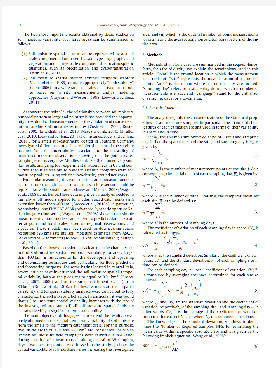
2.1.Statistical method

The analysis regards the characterization of the statistical prop-erties of soil moisture samples.In particular,the main statistical features of each campaign are analyzed in terms of their variability in space and in time.

Let h ijk the soil moisture observed at point i,site j and sampling day k,then the spatial mean of the site j and sampling day k,h jk,is given by:

h jk?

1

N p

X N p

i?1

h ijke1T

where N p is the number of measurement points at the site j.As a consequence,the spatial mean of each sampling day,h k,is given by:

h k?

1

N

X N

j?1

h jke2T

where N is the number of sites.Similarly,the temporal mean for each site,h j,can be de?ned as:

h j?

1

M

X M

k?1

h jke3T

where M is the number of sampling days.

The coef?cient of variation of each sampling day in space,CV k,is calculated as follows:

CV k

k

?

???????????????????????????????????????

1P N j?1eh jkàh kT2

q

k

e4T

where r k is the standard deviation.Similarly,the coef?cient of var-iation,CV j,and the standard deviation,r j,of each sampling site in time can be de?ned.

For each sampling day,a‘‘local’’coef?cient of variation,CV local

k

, is computed by averaging the ones determined for each site as follows:

CV local

k

?

1

N

X N

j?1

CV jk?

1

N

X N

j?1

h jk

!

e5T

where r jk and CV jk are the standard deviation and the coef?cient of variation,respectively,of the sampling site j and sampling day k.In

other words,CV local

k

is the average of the coef?cients of variation computed for each of N sites where N p measurements are done.

The knowledge of the standard deviation,r,allows to deter-mine the Number of Required Samples,NRS,for estimating the mean value within a speci?c absolute error and it is given by the following implicit equation(Wang et al.,2008):

NRS?t2

1àa=2;NRS-1

r2

AE

e6T

64L.Brocca et al./Journal of Hydrology422–423(2012)63–75

where t1àa/2,NRS-1is the value of the Student’s t-distribution at the con?dence level1àa/2and with NRS degrees of freedom,and AE is the absolute error expressed in volumetric soil moisture(%vol/ vol).

To determine the spatial variability of soil moisture as a func-tion of the dimension of the investigated area,the relationship pro-posed by Famiglietti et al.(2008)is employed:

VareST?CáS De7Twhere C is a parameter,D is a fractal power,S is area extension and Var(S)is the variance.Such a relationship can be used to estimate the average variance conditions at a particular scale and,hence,to have indications on the optimal number of soil moisture measure-ment sites as a function of spatial scale.

Then,the relationship between the standard deviation as well as coef?cient of variation and the areal mean soil moisture is inves-tigated.In fact,it was commonly found(see e.g.Bell et al.,1980; Famiglietti et al.,1999,2008;Jacobs et al.,2004;Choi et al., 2007;Brocca et al.,2007,2010a;Choi and Jacobs,2010)that a decreasing exponential law accurately describes the dependence between the coef?cient of variation and the mean and a convex up-ward relationship holds between standard deviation and mean. These relationships allow to characterize the soil moisture variabil-ity and,hence,to address the assessment of the NRS to estimate the mean value within an area with a prescribed absolute error as a function of the average soil moisture conditions.

Another important aspect,mainly linked to upscaling/down-scaling purposes,regards the characterization of the probability distribution describing soil moisture samples for different average soil moisture conditions.In the scienti?c literature,soil moisture samplings were frequently found or assumed as normally distrib-uted(Bell et al.,1980;Nyberg,1996;Anctil et al.,2002;Buttafuoco et al.,2005;Joshi and Mohanty,2010)even though,mainly for wet or dry conditions,some authors suggested that a more?exible dis-tribution(e.g.Beta distribution)might be more appropriate (Famiglietti et al.,1999;Ryu and Famiglietti,2005).In this study, four different theoretical probability distribution are tested: Normal,Lognormal,Gamma and Beta.

2.2.Temporal stability

The second part of the analysis concerns the temporal stability of the measured soil moisture values.This approach,?rstly pro-posed by Vachaud et al.(1985),allows:(i)to characterize the tem-poral persistence of spatial soil moisture pattern and(ii)to identify the sampling points(in our case the sampling sites)in which soil moisture can be considered as representative for the entire area of study.

Therefore,?rstly the temporal persistence analysis is carried out through the computation of the spatial correlation coef?cients between the soil moisture data of different sampling days.For each value the statistical signi?cance is veri?ed and,in addition,the time window for which soil moisture spatial patterns are persis-tent is also estimated.Then,the classical temporal stability analy-sis based on the parametric test of the relative differences is also conducted.Brie?y,the relative difference,d jk,at site j and sampling day k is given by:

d jk?

h jkàh k

k

e8T

For each site j,the mean,d j,and the standard deviation,r(d j),of the relative differences are:d j?

1

M

X M

k?1

d jke9T

red

j

T?

??????????????????????????????????????????

1X M

k?1

ed jkàd jT2

v u

u t

e10T

A‘‘representative’’point of the mean value in time is character-ized by a low value of j d j j and r(d j).

2.3.Random combination method

Finally,a random combination method is adopted to obtain the number of measurement points required to estimate,within a pre-de?ned accuracy,the temporal evolution of areal mean soil mois-ture(Wang et al.,2008;Brocca et al.,2010a).In particular,the method consists of the following steps:

1.randomly select n0point measurements(n0

able N observations in N r replicates;

2.for each replicate,the time series of areal mean soil moisture

are calculated,so obtaining N r soil moisture time series in total;

3.N r time series are statistically compared with the one based on

all N measurements sites(denoted as benchmark time series);

for that,the coef?cient of determination,R2,and the Root Mean Square Error,RMSE,are employed;

4.mean and standard deviation of the two above statistic mea-

sures(R2and RMSE)are assessed;

5.points1–4for n0ranging between1and N are repeated.

The mean and the standard deviation of each performance sta-tistic are expressed as a function of the number of measurement points.Therefore,once a threshold for the performance statistics is assumed,the analysis allows to address the optimization of an in situ soil moisture network.In fact,if previous soil moisture cam-paigns were available for the study area,the temporal stability would permit to select the best locations where to set up in situ sensors.However,if previous information were not available,the random combination method would address the determination of the error in the estimation of the areal mean soil moisture value when the sensors are randomly installed in a given region.There-fore,the combination of these two analyses(i.e.,temporal stability and random combination method)allows to obtain all the informa-tion required for the optimization of an in situ soil moisture network.

3.Study area and measurements

The soil moisture measurements were carried out for two areas in an inland region of central Italy,located in the Upper Tiber River Basin(see Fig.1),i.e.,the Trasimeno Lake catchment and the Genna and Caina catchments,indicated henceforth as LAGO and GENCAI, https://www.doczj.com/doc/9c7593145.html,GO is located around the biggest stretch of water of the Upper Tiber Valley,the Trasimeno Lake,and covers an area of 178km2.It shows a mean slope of5%,the predominant land use is cropland(70%)followed by woodland(15%).GENCAI is located to east side of LAGO and it covers an area of242km2;with pre-dominant land use of cropland(73%),urbanized(12%)and range-land(15%).The slope is a little bit higher than LAGO,with a mean value of9%.

The region is characterized by a Mediterranean semi-humid cli-mate with a mean annual precipitation of$900mm occurring mostly in the autumn-spring period.Mean annual temperature is 12°C and,accordingly,the mean annual potential evapotranspira-tion,computed with the Thornthwaite formula is almost800mm.

L.Brocca et al./Journal of Hydrology422–423(2012)63–7565

The near surface (0–15cm)volumetric soil moisture was sam-pled by a portable unit using a two wire connector-type time do-main re?ectometry (TDR)probe of the Soil Moisture equipment Corp.(1996)TRASE òTDR.The standard calibration curve (Skaling,1992)is applied to infer the volumetric soil moisture from the measured dielectric constant.The equipment has a quoted error of ±2%vol/vol or less.

The sampling scheme is the same for the two study areas:46sites were identi?ed (1site each 4–5km 2)and for each of them three measurement points were collected during a sampling day.In fact,previous studies (Brocca et al.,2009,2010a )found that three measurements might be suf?cient to characterize the soil moisture temporal pattern of the areal mean soil moisture within an area of $10km 2.Therefore,the sampling scheme can be consid-ered suitable to estimate the mean soil moisture value for an area of $200km 2,as investigated in this study.Fig.1shows the location of soil moisture measurements for the two areas along with the morphology of the territory.Overall,during each sampling day,a total of 138measurements of soil moisture were carried out for each area.These samplings were repeated from February 2009to January 2010with almost weekly frequency except for the summer months because of soil hardness.During the investigated period,the measurements in the two areas were carried out nearly during the same day thus obtaining 34and 35sampling days for LAGO and GENCAI,respectively.

For both study areas Table 1summarizes the main characteris-tics of the selected sampling sites in terms of soil texture (as de-rived by a detailed geo-lithological map)and terrain.As it can be seen,for LAGO area two different and contrasting soil texture clas-ses are predominant,i.e.,loamy sand and silty clay for 50.0%and

37.0%of sites,respectively.On the other hand,for GENCAI the dis-tribution of soil texture classes is slightly more uniform.The ter-rain of the sites is mostly ?at (56.5%of sites with slope <5%)even though several sites located on hillslopes (slope >15%)were also monitored (7.6%of sites).As regards the land use,the choice of the measurement sites was based on the criterion of minimum interaction with human activities,such as tillage,thus selecting grassland and bare soil sites.

The scheme adopted for the sampling campaigns assumes par-ticular importance because of its wide spatial and temporal cover-age;in fact,to our knowledge,it is one of the ?rst attempts investigating soil moisture variability with in situ observations covering large areas (>150km 2)for a period of almost a year with high resolution both in space and in time.Previous studies have fo-cused their attention on the design of the measurements campaign either favouring the spatial aspects or the temporal one,but never considering both of them.In our case,the long and frequent sam-pling allows to analyze the entire range of variability of soil mois-ture,from dry to wet conditions.Moreover,the large areal extension permits to characterize soil moisture variability at the appropriate scale useful both for hydrological studies and for the validation of soil moisture estimates from remote sensing.

4.Results and discussions

In the following,?rstly the main statistical features of the soil moisture sampling campaign are investigated.Then,the results obtained by applying the statistical,temporal stability and random combination analysis are discussed for each study area.

A

two study areas (Trasimeno Lake area on the left,LAGO,Genna and Caina area on the right,GENCAI)with the in each area)and the terrain morphology.

comparison with the?ndings obtained by previous studies carried

out in the same study area and in other regions is also performed.

4.1.Statistical analysis

The statistical descriptors of the approximately10,000mea-surements of soil moisture performed in the two areas are here analyzed.In Table2,the main statistical descriptors for each sam-pling day are listed including also the third and fourth statistical moments(skewness and kurtosis)and the v2values of the Pear-son’s test for normality.

A preliminary investigation of the temporal evolution of the areal mean soil moisture is performed.As can be seen in Fig.2; the two investigated areas display a very similar behavior,mainly linked to rainfall pattern.Analogously,the coef?cient of variation (and the standard deviation)of the two areas show the same trend with increasing values with drier soil conditions(Table2).A direct comparison between the two areas is also carried out by consider-ing only the concurrent sampling days(28in total).As expected,a very good agreement between the two areal mean soil moisture sequences is detected,with a correlation coef?cient,r,equal to 0.92and a Root Mean Square Error,RMSE,of about3.72%vol/vol. Its worth noting that also the standard deviations and the coef?-cients of variation display a fairly good correspondence,with r equal to0.31and0.83,respectively(both signi?cant at95%con?-dence level).This?rst comparison reveals that the overall study re-gion,whose total size is$420km2,presents a very similar soil moisture temporal pattern not only in terms of mean values but also in terms of variability(as expressed by standard deviation and coef?cient of variation).

4.1.1.Coef?cient of variation

The spatial and temporal soil moisture variability is investi-gated by considering the coef?cient of variation computed in space,CV k,and in time,CV j.The coef?cient of variation is used as statistical descriptor because it allows to compare the variability of different samples even though characterized by different mean values,and,hence,to analyze the soil moisture variability across different spatial scales.For both areas,the spatial CV k is found fairly low,never exceeding0.37(Table2),and on average equal to0.21.On the other hand,the temporal CV j is found to be equal, on average,to0.33and0.35for GENCAI and LAGO,respectively, slightly higher than the value of$0.30obtained by Brocca et al. (2010a)for a smaller study area($60km2).These results con?rm that the soil moisture temporal variability is more signi?cant than the spatial one and,hence,practical indications about the optimal monitoring of this variable can be derived.

Moreover,the spatial CV local

k

is found on average equal to$0.08 (with a maximum value of0.18)and considerably lower than CV k.

The?ndings about CV k and CV local

k

suggest,as expected,an increase of soil moisture variability with area extension.

Another interesting link is established between the values for the whole area and the local ones,i.e.CV k versus CV local

k

.In fact, as displayed in Fig.3,the two datasets tend to arrange themselves linearly,indicating an almost constant ratio between local and glo-bal spatial variability.This means that when the spatial variability of the whole area is high,the same occurs at local scale despite of the very different spatial extent($200km2versus$1m2).These ?ndings are much evident for LAGO area,with a ratio between glo-bal and local values equal to3;for GENCAI area the ratio reduces to 2.These differences can be related to the higher soil heterogene-ities of the LAGO area(see Table1).

More interestingly,taking also account of the information re-ported in the previous studies conducted in the same region and reported in Table3(Brocca et al.,2007,2009,2010a),the relation between the spatial variability of soil moisture and the dimension of the investigated area can be investigated further.Speci?cally, the spatial CV k increases with the area,with average values equal to:(i)0.06–0.08at local scale(1–500m2),(ii)0.10at small plot scale(501–5000m2),(iii)$0.15at plot scale(5001–100,000m2), and(iv)$0.20for larger areas(50–250km2).As concerns the var-iance,equation(7)is applied obtaining a value of the fractal power parameter,D,equal to$0.16,which is twice the value obtained by Famiglietti et al.(2008),who analyzed the relationship between variance and extent scale between$200m2and4km2.Obviously, the different increase of variance with the extent scale depends on the speci?c conditions of the investigated areas as well as to the differences in the sampling depth.In fact,Famiglietti et al.(2008) considered soil moisture data collected at0–5cm depth that are usually characterized by a higher variability than that referring to the0–15cm depth analyzed here.If compared with the standard deviation values given in Famiglietti et al.(2008),the values ob-tained for central Italy sites are50%lower.Overall,these?ndings furnish a clear indications about the spatial variability of soil mois-ture at different scales in central Italy and,clearly,also for similar regions across the world.Such results can be used to estimate the average variance conditions at a desired scale and,consequently, the Number of Required Samples(NRS).For instance,by combining Eqs.(6)and(7)the NRS as a function of the area can be easily com-puted and it is found to be equal to8,18and27for an area of1, 100and1000km2,respectively,by assuming an absolute error of ±2%vol/vol and a con?dence level of95%.

4.1.2.Relationship between statistical descriptors

An important aspect in the analysis of soil moisture spatial var-iability is the relationship between the areal mean soil moisture, h k,the corresponding standard deviation,r k,and the coef?cient of variation,CV k.For LAGO and GENCAI areas these relationships are shown in Fig.4a–d.We note that the solid lines displayed in the?gures are computed by?tting the relationship between CV k and h k with an exponential law,CV k?AáexpeàB h kT,in accordance with previous studies(e.g.Famiglietti et al.,2008;Brocca et al.,

Table1

Main characteristics of the two investigated areas and of the soil moisture sampling campaigns.

Area Soil texture Terrain Size(km2)Measurement period NSD NSS class%sites slope%sites

LAGO Loamy sand50.0<560.8178February2009–January20103446 Loam 2.25–1019.6

Clay loam10.810–1510.9

Silty clay37.0>158.7

GENCAI Loamy sand30.4<552.2242February2009–December20093546 Loam12.85–1023.9

Clay loam17.710–15%17.4

Silty clay39.1>15% 6.5

NSD:number of sampling days.NSS:number of sampling sites.

L.Brocca et al./Journal of Hydrology422–423(2012)63–7567

68L.Brocca et al./Journal of Hydrology422–423(2012)63–75

Table2

Main statistical properties of the soil moisture data collected during the sampling campaign in the two study areas.

Date Mean(%)r(%)CV Range(%)25°p.(%)75°p.(%)Kurtosis Skewness v2

LAGO

25/02/200932.4 5.560.1722.7–47.128.634.9 3.430.91 6.9* 13/03/200930.4 4.950.1624.0–47.626.532.1 5.11 1.3010.3* 17/03/200928.1 4.490.1620.5–39.525.431.0 3.040.528.6* 24/03/200930.2 4.780.1622.5–44.827.432.3 4.030.858.3* 01/04/200935.5 6.150.1727.5–50.331.339.2 2.600.8829.5a 07/04/200928.4 3.580.1320.3–38.025.629.9 3.930.797.9* 16/04/200922.3 4.960.2214.1–32.017.926.2 1.890.22 4.8* 23/04/200932.0 4.860.1524.6–45.328.833.8 3.80 1.118.3* 07/05/200927.6 6.070.2217.0–43.223.931.4 3.520.62 5.1* 13/05/200919.3 5.140.2712.2–31.115.023.3 2.030.4713.8** 19/05/200915.7 4.390.289.2–25.612.319.1 2.360.6813.8** 26/05/200915.0 3.700.2510.1–23.212.118.0 2.500.7413.8** 05/06/200928.6 3.810.1321.4–38.925.530.9 3.180.388.3* 11/06/200924.0 3.460.1415.3–30.822.027.2 2.62à0.3010.3* 17/06/200916.2 4.500.287.1–26.312.919.6 2.470.35 4.8* 24/06/200915.9 4.790.307.8–27.912.320.6 2.510.51 6.5* 03/07/200923.4 5.520.248.3–32.420.327.4 2.89–0.65 5.8* 08/07/200922.6 5.760.2511.1–34.117.926.5 2.08à0.3217.3* 15/07/200913.2 4.050.31 5.9–24.710.315.3 3.160.47 2.7* 22/07/200913.6 5.060.37 6.8–29.09.515.0 4.52 1.1913.1** 08/09/20098.1 2.400.30 4.2–14.7 6.29.7 2.750.70 5.5* 17/09/200916.3 4.690.299.1–28.312.320.6 2.370.5616.6** 22/09/200921.2 5.210.258.2–29.118.125.6 2.49à0.56 5.1* 02/10/200911.3 3.970.35 6.2–20.98.014.1 2.880.7613.5** 16/10/200920.6 5.330.269.5–30.416.625.0 2.18à0.1812.4** 30/10/200924.9 5.240.2114.5–36.121.328.8 2.34à0.249.0* 11/11/200928.0 4.190.1517.3–37.926.029.8 3.60à0.068.3* 18/11/200925.2 4.080.1615.2–33.122.128.2 2.63à0.26 6.2* 25/11/200927.0 3.990.1517.2–33.425.430.0 3.44à0.85 6.9* 02/12/200933.5 3.720.1126.0–41.530.736.4 2.310.28 5.5* 16/12/200930.7 3.720.1222.9–38.728.432.5 2.760.07 4.1* 14/01/201033.5 3.390.1026.1–40.731.335.3 2.52à0.07 5.5* 20/01/201031.5 3.830.1226.5–40.428.334.7 2.080.5212.8** 27/01/201033.8 3.350.1027.2–42.631.736.3 2.720.12 4.1*

GENCAI

24/02/200937.6 5.720.1526.7–51.532.740.1 2.630.2611.0* 03/03/200944.3 5.710.1333.8–53.938.448.5 2.00à0.5013.1** 12/03/200933.4 4.130.1223.3–42.830.036.2 2.70à0.2610.0* 17/03/200929.5 3.840.1318.1–36.226.831.6 3.23à0.28 3.7* 24/03/200930.9 3.630.1224.2–38.427.934.8 2.090.18 3.7* 01/04/200936.3 4.260.1225.6–44.534.139.3 2.68à0.33 2.0* 07/04/200931.3 3.600.1222.0–39.128.734.2 2.98à0.33 4.8* 16/04/200927.0 4.190.1617.5–36.024.130.0 2.840.00 2.7* 23/04/200930.3 3.620.1221.9–38.527.733.3 2.410.01 6.2* 07/05/200930.9 5.620.1820.2–45.926.935.3 2.720.42 4.1* 21/05/200918.6 5.730.318.3–31.913.824.1 2.170.3110.3* 28/05/200917.3 4.680.278.2–26.114.021.1 2.120.3813.5** 04/06/200935.6 5.620.1625.3–47.331.238.9 2.280.0312.8** 12/06/200924.5 5.380.2212.8–37.020.127.5 2.610.14 2.0* 18/06/200919.6 5.500.2811.0–30.415.324.6 1.850.3114.5** 25/06/200916.3 5.020.317.3–25.313.119.8 2.040.18 5.5* 02/07/200925.6 5.820.2314.1–36.222.130.7 2.24à0.18 5.5* 11/07/200921.2 5.980.2812.3–34.615.426.1 2.090.317.6* 17/07/200917.6 5.590.3210.0–33.914.020.9 3.480.91 6.2* 24/07/200914.6 3.700.259.2–24.412.215.9 3.58 1.027.2* 09/09/200913.1 3.060.23 6.0–21.211.214.8 3.540.29 1.3* 18/09/200924.6 6.300.269.4–36.021.230.1 2.52à0.41 3.4* 23/09/200928.4 6.000.2113.6–37.024.233.2 2.68à0.66 6.2* 30/09/200917.6 6.180.35 5.3–29.012.922.6 2.11à0.01 3.7* 08/10/200914.7 4.880.33 5.9–26.411.517.9 3.060.60 3.7* 14/10/200919.5 5.530.289.4–29.715.124.4 1.910.3012.4** 21/10/200918.0 5.170.298.9–29.014.721.1 2.710.488.3* 28/10/200921.3 5.680.2712.1–34.717.324.1 2.730.44 4.1* 04/11/200926.3 5.770.2214.6–36.521.531.1 1.93à0.18 5.5* 12/11/200929.3 6.090.2114.7–48.927.131.4 5.730.7113.5** 19/11/200925.6 4.120.1612.8–33.223.627.6 4.20à0.76 3.4* 30/11/200933.2 3.750.1125.2–38.630.536.2 2.34à0.57 5.8* 07/12/200933.8 4.050.1226.2–41.330.637.2 1.98à0.1010.7* 10/12/200931.9 3.710.1223.8–40.629.135.1 2.64à0.08 6.2* 18/12/200933.1 4.310.1325.1–41.029.536.4 1.96à0.11 4.1*

r:standard deviation,CV:coef?cient of variation,v2:chi square values of the Pearson’s test.

*Normal at5%signi?cance level.

**Normal at1%signi?cance level.

a Non normal.

2010a ).In Fig.4a and b the same relationship is employed,i.e.,r k ?CV k áh k ?A áexp eàB h k Táh k ;thus the solid line does not repre-sent the best ?t line relationship between r k and h k .As it was ob-served in previous analyses of ?eld campaigns data (e.g.Teuling and Troch,2005;Lawrence and Hornberger,2007;Teuling et al.,2007;Famiglietti et al.,2008;Pan and Peters-Lidard,2008;Brocca et al.,2010a;Choi and Jacobs,2010;Tague et al.,2010)and through

Choi and Jacobs,2010;Tague et al.,2010),highlights that areas of similar extent are characterized by very similar values of the B coef-?cient,that vary in the range 0.02–0.09,implying the same decreas-ing pattern in the relation CV k versus h k .It is worth noting that in most of the previous investigations the relationship between h k and CV k refer to a limited temporal windows (2–3months)and to areas located in the central states of America,characterized by a dif-ferent climate.

3.Relationship between the spatial coef?cient of variation computed for area,CV k ,and the average of the local ones computed for each site,CV local k two investigated areas.

Table 3

Summary of the main characteristics of the previous soil moisture campaigns (Brocca et al.,2007,2009,2010a )carried out in the same region of the study area.Site name Soil texture Size Measurement period

NSD NSS Ponte della Pietra Silty clay 405m 2August 2002–September 20021445Ponte della Pietra Silty clay

9m 2

October 2002

3100Ingegneria Silty clay loam 5000m 2February 2004–April 20041450Colorso Sandy loam 8800m 2October 2002–January 20067108Colorso Sandy loam

400m 2April 2005

1121CRI (VAL1)Silty clay and sand 3000m 2November 2006–November 20073530COL (VAL2)Alluvial deposit 3000m 2November 2006–November 20073530LEC (VAL3)Alluvial deposit 3000m 2November 2006–November 20073530CBE (VAL4)Sandy loam 3000m 2November 2006–November 20073530VRO (VAL5)Alluvial deposit 3000m 2November 2006–November 20073530MOL (VAL6)Gravel

3000m 2November 2006–November 20073530MON (VAL7)Sandy loam 3000m 2November 2006–November 20073530Vallaccia a

–

$60km 2

November 2006–November 2007

35

7

NSD:number of sampling days,NSS:number of sampling sites.a

Measurements carried out at seven sites (VAL1–VAL7)are assumed representative of the soil moisture behavior for the Vallaccia area.

Moreover,we note that at local scale(i.e.considering r local

k

and

CV local

k

versus h k)an exponential decreasing trend for the coef?cient of variation,and a convex upward relationship for the standard deviation is also detected,thus con?rming that the relationships between the main statistical descriptors at local and global scales are characterized by very similar behavior.

The observed decreasing trend between h k and CV k allowed to quantify the NRS as a function of the average wetness conditions. Assuming the relationship between h k and CV k to be represented by the exponential law previously mentioned,the NRS is deter-mined in relation to the areal mean soil moisture and to a pre?xed con?dence level(Jacobs et al.,2004;Brocca et al.,2010a).For a con?dence level of95%and an absolute error,AE,±2%,±4%and ±6%vol/vol,the NRS as a function of h k is shown in Fig.5.For both areas and AE±2%vol/vol,the NRS is less than26,a slightly lower value than that obtained by Brocca et al.,2010a for the Vallaccia catchment(see Table3)in central Italy(equal to40).However, the NRS obtained in this study matches with those reported in the scienti?c literature;in fact,a NRS between15and40has been usually obtained for soil moisture sampling campaigns conducted in different climatic and geomorphological conditions(Famiglietti et al.,2008).The maximum value for NRS(equal to26)obtained here is a further con?rmation of the goodness of the design of the soil moisture campaign used for this study for which46sites were monitored.If higher AE is considered,the NRS strongly re-duces with maximum values equal to only3and1for AE±4% and±6%vol/vol,respectively.

The maximum NRS value obtained through the statistical anal-ysis referring to an AE lower than±2%vol/vol for95%cases,can be considered to set up a reliable in situ monitoring network ad-dressed to the validation of satellite soil moisture retrieval algo-rithms and sensors.In fact,for this type of application the in situ soil moisture observations should represent the benchmark values for the validation of the satellite estimates.Instead,if in situ soil moisture data are?nalized to improve and test rainfall-runoff modeling,the‘‘average’’error is more meaningful and a different performance metric as,for instance,the Root Mean Square Error, RMSE,computed on the soil moisture temporal pattern should be used for determining NRS.As shown in the following sections, for this type of application the NRS strongly reduces.

between areal mean soil moisture and(a and b)standard deviation,(c and d)coef?cient of variation for:(a and c)LAGO, coef?cient of variation versus the mean are also shown as solid lines.

4.1.3.Probability distribution

Another important issue of the statistical analysis is the knowl-edge of the probability distribution of soil moisture,which allows to establish its variability within remote sensing footprints or within a cell of a distributed hydrological model.Referring to the v 2values of the Pearson’s test and considering a signi?cance level of 5%,we observed that for 71%and 83%sampling days of LAGO and GENCAI area,respectively,a normal probability distribution can be used (Choi and Jacobs,2007).As regards the other three probability distributions analyzed in this study,i.e.,Lognormal,Gamma and Beta,for LAGO area the best results are obtained for the Gamma and Lognormal probability distribution for which 79%and 82%sampling days pass the Pearson’s test.For GENCAI area,the Gamma and Beta distributions are the two more suitable with 91%(for both of them)of sampling days that pass the Pear-son’s test.

To further investigate if for dry or wet conditions a different probability distribution could be more appropriate to describe soil moisture samplings,the sampling days of LAGO and GENCAI areas are subdivided in three subsets according to the mean soil mois-ture values;i.e.,dry (<20%vol/vol),intermediate (between 20%and 30%vol/vol)and wet (>30%vol/vol)conditions.The size of the three subset is nearly the same for both LAGO and GENCAI areas with 11–14samples for each subset.Then,for each subset the average v 2values are computed and compared among the dif-ferent statistical distributions.For GENCAI area,in accordance with previous studies (Famiglietti et al.,1999;Ryu and Famiglietti,2005),the best probability distribution is the normal for interme-diate conditions (average v 2value equal to 5.96),the Beta distribu-

2 4.2.Temporal stability analysis

The spatial correlation coef?cient,r ,between soil moisture data of different sampling days is ?rstly investigated.A representation of the data is shown in Fig.6for both areas;wherein dark cells im-ply high correlation values.It can be seen that during the winter and the summer seasons,for which the mean soil moisture keeps on almost constant,correlation values are quite high (r >0.7)also for samplings separated by several weeks.In fact,considering a sig-ni?cance level equal to 0.001(threshold r -value equal to 0.47),during the winter season the spatial correlation keeps on signi?-cant for sampling days separated by nearly two months;in sum-mer this period reduces to 1.5months.More interestingly,the samplings carried out in winter are signi?cantly correlated even in the case that they are separated by more than 8months.This can be seen in Fig.6by considering,for instance,the high r -values obtained for the LAGO area between the measurements of 25th February,2009and of 14th or 20th January,2010.Instead,in the transition period between dry and wet conditions (or viceversa)the correlation values strongly decrease (r <0.3),especially from dry to wet conditions.These results are in accordance with previ-ous studies (Mohanty and Skaggs,2001;Cosh et al.,2004;Fernan-dez and Ceballos,2005)and provide further insights for addressing the soil moisture monitoring.In fact,the estimation of soil mois-ture spatial pattern during transition periods reveals to be more dif?cult and,hence,in these conditions its use for modeling pur-poses (hydrological,meteorological,agricultural,etc.)will provide higher uncertainties (Zehe and Bloschl,2004).

As far as the classical parametric test of the relative differences L.Brocca et al./Journal of Hydrology 422–423(2012)63–7571

of d j and r (d j ).In this study,we selected as representative site the one with the lowest r (d j )among the ones with d j <5%;based on this criterion the site ‘‘34’’and ‘‘36’’are the two most representa-tive site for LAGO and GENCAI area,respectively (see Fig.1for the location of these sites).For each study area,Fig.8shows the

temporal variability of a single site allows to explain,on average,nearly 80%of that observed for the whole area.As expected,the performances are lower than those reported in Brocca et al.(2010a)who obtained average R 2-values in the range 0.80–0.93,likely due to the larger areas investigated in the present study.On the other hand,Ali and Roy (2010)obtained lower R 2-values (in the range 0.32–0.91)for soil moisture measurements collected at a 5.1ha forested catchment located in Canada.Therefore,once again,the heterogeneities in the soil and land use characteristics is con?rmed to affect the capability to extrapolate point measure-ments to larger areas.However,in the study area,if only the tem-poral trend of soil moisture has to be captured,as,for instance,for being assimilated into a hydrological or meteorological model (Koster et al.,2009;Entekhabi et al.,2010),even a single site can be considered enough.

A more in-depth analysis is conducted by applying the random combination methodology.The analysis is performed by selecting

Comparison of the areal mean soil moisture versus the soil moisture observed at the ‘‘representative’’site for the two study areas.

Table 4

Mean,maximum and minimum determination coef?cient,R 2,and Root Mean Square Error,RMSE,between the benchmark time series of the areal mean soil moisture and the time series obtained at each of the 46sites in the two investigated areas.Area

R 2RMSE (%vol/vol)Mean

Maximum Minimum Mean Maximum Minimum LAGO 0.8120.9110.510 4.3197.970 2.271GENCAI

0.788

0.900

0.486

4.908

6.953

3.029

from1to20sites(out of46)for N r=1000replicates and then com-paring the time series of the spatial mean soil moisture values ob-tained from these sites with the benchmark soil moisture.For the two study areas,Fig.9shows the R2and the RMSE computed be-tween the benchmark soil moisture time series and the one ob-tained by averaging a different number of sites(randomly selected)against the number of measurements per100km2.If an accuracy of2%vol/vol is required,only2sites per100km2are needed to obtain the areal mean soil moisture pattern with an R2 equal to$0.95.Moreover,for a number of sites per100km2great-er than5the increase in the accuracy is not signi?cant.These re-sults suggest that a slightly coarse in situ monitoring network(1 station per50km2)in the study area should be able to capture the mean soil moisture temporal pattern with very high accuracy (Miralles et al.,2010;Loew and Schlenz,2011).

5.Conclusions

Near-surface soil moisture measurements carried out over1-year period,with an almost weekly frequency,in two adjacent areas of central Italy have been used to investigate the soil mois-ture variability at medium catchment scale($150km2)and to ad-dress the monitoring of this hydrological variable at large scales. Based on the analysis and the results obtained for the investigated study area,the following conclusions can be drawn:

(i)the temporal variability of soil moisture is more signi?cant

than the spatial one as expressed by the analysis of the tem-poral and spatial coef?cients of variation;

(ii)on the basis of observations carried out in the study area,the soil moisture variability increases with the extent of the investigated area up to an area of$10km2con?rming?nd-ings of previous studies(Brocca et al.,2007,2009,2010a);

for greater extents the spatial coef?cient of variation remains quite constant and equal to0.21;

(iii)the probability distribution followed by soil moisture sam-ples can be assumed as normal for77%of cases but in wet and dry conditions a different probability distribution seems to be more appropriate(Gamma and Lognormal);

(iv)local(1–2m2)and global($200km2)soil moisture mea-surements are characterized by a very similar behavior,i.e.

the local variability increases with the global one;

(v)also for areas of$200km2,soil moisture?eld exhibits tempo-ral stability,in fact,one representative site is able to estimate the areal mean value with a determination coef?cient higher than0.88and root mean square error less than3%vol/vol;

(vi)overall,in the investigated area,2measurement sites per 100km2randomly selected are suf?cient to estimate the areal mean temporal pattern with a root mean square error less than2%vol/vol.

The capability to upscale point measurements for areas greater than100km2is in good agreement with the?ndings by Miralles et al.(2010)and Loew and Schlenz(2011),who reached the same conclusions by investigating the errors associated to the upscaling of point-scale observations aimed at validating coarse resolution satellite estimates.

Moreover,the obtained results can be effectively employed to address the use of soil moisture data for hydrological and others applications.For instance,they have been used to design an in situ network of soil moisture sensors operating in real-time that is going to be set up in the Upper Tiber River basin($5000km2)to improve the knowledge of the rainfall-runoff transformation pro-cesses and to support the National Civil Protection activities re-lated to real-time?ood prediction and forecasting.

Further investigations are still needed to clearly assess the ef-fects of heterogeneities of land use,soil properties and topography on soil moisture spatial–temporal variability.Also the analysis of deeper layers,likely characterized by a different hydrological behavior,should be performed to reach general conclusions for the whole root-zone pro?le.

Acknowledgments

The authors wish to thank R.Rosi for his assistance.This work was funded by the National Research Council of Italy and by the Italian Ministry of Education,University and Research(special Pro-ject‘‘Assimilazione di osservazioni remote e al suolo per la calibr-azione di modelli idrologici distribuiti e la previsione delle piene improvvise’’).

References

Albergel,C.,Calvet,J.C.,de Rosnay,P.,Balsamo,G.,Wagner,W.,Hasenauer,S., Naeimi,V.,Martin, E.,Bazile, E.,Bouyssel, F.,Mahfouf,J.F.,2010.Cross-evaluation of modelled and remotely sensed surface soil moisture with in situ data in Southwestern France.Hydrol.Earth Syst.Sci.14,2177–2191.

doi:10.5194/hess-14-2177-2010.

Albertson,J.D.,Montaldo,N.,2003.Temporal dynamics of soil moisture variability:

1.Theorethical basis.Water Resour.Res.39(10),1274.doi:10.1029/

2002WR001616.

Ali,G.A.,Roy,A.G.,2010.A case study on the use of appropriate surrogates for antecedent moisture conditions(AMCs).Hydrol.Earth Syst.Sci.14,1843–1861.

doi:

10.5194/hess-14-1843-2010.

Anctil, F.,Mathieu,R.,Parent,L.E.,Viau, A.A.,Sbih,M.,Hessami,M.,2002.

Geostatistics of near-surface moisture in bare cultivated organic soils.J.

Hydrol.260,30–37.doi:10.1016/S0022-1694(01)00600-X.

Bell,K.R.,Blanchard,B.J.,Schmugge,T.J.,Witczak,M.W.,1980.Analysis of surface moisture variations within large?eld sites.Water Resour.Res.16,796–810.

doi:10.1029/WR016i004p00796.

Bolten,J.D.,Crow,W.T.,Jackson,T.J.,Zhan,X.,Reynolds,C.A.,2010.Evaluating the utility of remotely-sensed soil moisture retrievals for operational agricultural drought monitoring.IEEE J.Sel.Topics Appl.Earth Observ.3,57–66.

doi:10.1109/JSTARS.2009.2037163.

Brocca,L.,Morbidelli,R.,Melone,F.,Moramarco,T.,2007.Soil moisture spatial variability in experimental areas of Central Italy.J.Hydrol.333,356–373.

doi:10.1016/j.jhydrol.2006.09.004.

Brocca,L.,Melone,F.,Moramarco,T.,Morbidelli,R.,2009.Soil moisture temporal stability over experimental areas of Central Italy.Geoderma148(3–4),364–374.doi:10.1016/j.geoderma.2008.11.004.

Brocca,L.,Melone, F.,Moramarco,T.,Morbidelli,R.,2010a.Spatial-temporal variability of soil moisture and its estimation across scales.Water Resour.

Res.46,W02516.doi:10.1029/2009WR008016.

Brocca,L.,Melone,F.,Moramarco,T.,Wagner,W.,Hasenauer,S.,2010b.ASCAT Soil Wetness Index validation through in situ and modeled soil moisture data in central Italy.Remote Sens.Environ.114(11),2745–2755.doi:10.1016/ j.rse.2010.06.009.

Brocca,L.,Melone,F.,Moramarco,T.,Wagner,W.,Naeimi,V.,Bartalis,Z.,Hasenauer, S.,2010c.Improving runoff prediction through the assimilation of the ASCAT soil moisture product.Hydrol.Earth Syst.Sci.14,1881–1893.doi:10.5194/hess-14-1881-2010.

Brocca,L.,Hasenauer,S.,Lacava,T.,Melone,F.,Moramarco,T.,Wagner,W.,Dorigo, W.,Matgen,P.,Martínez-Fernández,J.,Llorens,P.,Latron,J.,Martin,C.,Bittelli, M.,2011.Soil moisture estimation through ASCAT and AMSR-E sensors:an intercomparison and validation study across Europe.Remote Sens.Environ.

115,3390–3408,doi:10.1016/j.rse.2011.08.003.

Buttafuoco,G.,Castrignano,A.,Busoni,E.,Dimase,A.C.,2005.Studying the spatial structure evolution of soil water content using multivariate geostatistics.J.

Hydrol.311,202–218.doi:10.1016/j.jhydrol.2005.01.018.

Calamita,G.,Brocca,L.,Perrone,A.,Piscitelli,S.,Lapenna,V.,Melone,F.,Moramarco, T.,submitted for publication.Electrical resistivity and TDR methods for soil moisture estimation in Central Italy test-sites.J.Hydrol.

Chen,Y.,2006.Letter to the editor on‘‘Rank Stability or Temporal Stability.Soil Sci.

Soc.Am.J.70,306.doi:10.2136/sssaj2005.0290.

Choi,M.,Jacobs,J.M.,2007.Soil moisture variability of root zone pro?les within SMEX02remote sensing footprints.Adv.Water Resour.30(4),883–896.

doi:10.1016/j.advwatres.2006.07.007.

Choi,M.,Jacobs,J.M.,2010.Spatial soil moisture scaling structure during soil moisture experiment2005.Hydrol.Process.25,926–932.doi:10.1002/ hyp.7877.

Choi,M.,Jacobs,J.M.,Cosh,M.H.,2007.Scaled spatial variability of soil moisture ?elds.Geophys.Res.Lett.34,L01401.doi:10.1029/2006GL028247.

Cosh,M.H.,Jackson,T.J.,Bindlish,R.,Prueger,J.H.,2004.Watershed scale temporal and spatial stability of soil moisture and its role in validating satellite estimates.

Remote Sens.Environ.92,427–435.doi:10.1016/j.rse.2004.02.016.

De Lannoy,G.J.M.,Houser,P.R.,Verhoest,N.E.C.,Pauwels,V.R.N.,Gish,T.J.,2007.

Upscaling of point soil moisture measurements to?eld averages at the OPE3 test site.J.Hydrol.343(1–2),1–11.doi:10.1016/j.jhydrol.2007.06.004.

De Wit,A.J.W.,van Diepen, C.A.,2007.Crop model data assimilation with the Ensemble Kalman?lter for improving regional crop yield forecasts.Agric.Forest Meteorol.146(1–2),38–56.doi:10.1016/j.agrformet.2007.05.004. Entekhabi,D.,1995.Recent advances in land-atmosphere interaction research.Rev.

Geophys.33,995–1003.doi:10.1029/95RG01163.

Entekhabi,D.,Reichle,R.H.,Koster,R.D.,Crow,W.T.,2010.Performance metrics for soil moisture retrievals and application requirements.J.Hydrometeorol.11, 832–840.doi:10.1175/2010JHM1223.1.

Entin,J.K.,Robock, A.,Vinnikov,K.Y.,Hollinger,S.E.,Liu,S.,Namkai, A.,2000.

Temporal and spatial scales of observed soil moisture variations in the extratropics.J.Geophys.Res.105,865–877.doi:10.1029/2000JD900051. Famiglietti,J.S.,Devereaux,J.A.,Laymon,C.A.,Tsegaye,T.,Houser,P.R.,Jackson,T.J., Graham,S.T.,Rodell,M.,van Oevelen,P.J.,1999.Ground-based investigation of soil moisture variability within remote sensing footprints during the Southern Great Plains1997(SGP97)Hydrology Experiment.Water Resour.Res.35,1839–1851.doi:10.1029/1999WR900047.

Famiglietti,J.S.,Ryu,D.,Berg,A.A.,Rodell,M.,Jackson,T.J.,2008.Field observations of soil moisture variability across scales.Water Resour.Res.44,W01423.

doi:10.1029/2006WR005804.

Fernandez,J.M.,Ceballos,A.,2005.Mean soil moisture estimation using temporal stability analysis.J.Hydrol.312,28–38.doi:10.1016/j.jhydrol.

2005.02.007.

Grayson,R.B.,Western,A.W.,1998.Towards areal estimation of soil water content from point measurements:time and space stability of mean response.J.Hydrol.

207,68–82.doi:10.1016/S0022-1694(98)00096-1.

Hu,W.,Shao,M.,Han,F.,Reichardt,K.,Tan,J.,2010.Watershed scale temporal stability of soil water content.Geoderma158(3–4),181–198.doi:10.1016/ j.geoderma.2010.04.030.

Hupet,F.,Vanclooster,M.,2002.Intraseasonal dynamics of soil moisture variability within a small agricultural maize cropped?eld.J.Hydrol.261,86–101.

doi:10.1016/S0022-1694(02)00016-1.Jacobs,J.M.,Mohanty, B.P.,En-Ching,H.,Miller, D.,2004.SMEX02:?eld scale variability,time stability and similarity of soil moisture.Remote Sens.Environ.

92,436–446.doi:10.1016/j.rse.2004.02.017.

Joshi,C.,Mohanty,B.P.,2010.Physical Controls of Near-Surface Soil Moisture across Varying Spatial Scales in an Agricultural Landscape during SMEX02.Water Resour.Res.46,W12503.doi:10.1029/2010WR009152.

Koster,R.D.the GLACE Team,2004.Regions of strong coupling between soil moisture and precipitation.Science305,1138–1140.doi:10.1126/ science.1100217.

Koster,R.D.,Guo,Z.,Yang,R.,Dirmeyer,P.A.,Mitchell,K.,Puma,M.J.,2009.On the nature of soil moisture in land surface models.J.Clim.22,4322–4335,215.doi:

10.1175/2009JCLI2832.1.

Koster,R.D.,Mahanama,S.P.P.,Livneh,B.,Lettenmaier,D.P.,Reichle,R.H.,2010.Skill in stream?ow forecasts derived from large-scale estimates of soil moisture and snow.Nat.Geosci.3,613–616.doi:10.1038/ngeo944.

Lawrence,J.E.,Hornberger,G.M.,2007.Soil moisture variability across climate zones.Geophys.Res.Lett.34,L20402.doi:10.1029/2007GL031382.

Loew, A.,Mauser,W.,2008.On the disaggregation of passive microwave soil moisture data using a priori knowledge of temporally persistent soil moisture ?elds.IEEE Trans.Geosci.Remote Sens.46(3),819–834.doi:10.1109/ TGRS.2007.914800.

Loew,A.,Schlenz,F.,2011.A dynamic approach for evaluating coarse scale satellite soil moisture products.Hydrol.Earth Syst.Sci.15,75–90.doi:10.5194/hess-15-75-2011.

Mascaro,G.,Vivoni, E.R.,Deidda,R.,2010.Downscaling soil moisture in the southern Great Plains through a calibrated multifractal model for land surface modeling applications.Water Resour.Res.46,W08546.doi:10.1029/ 2009WR008855.

Matgen,P.,Heitz,S.,Hasenauer,S.,Hissler,C.,Brocca,L.,Hoffmann,L.,Wagner,W., Savenije,H.H.G.,in press.On the potential of METOP ASCAT-derived soil wetness indices as a new aperture for hydrological monitoring and prediction:a ?eld evaluation over Luxembourg.Hydrol.Process.doi:10.1002/hyp.8316. Merlin,O.,Walker,J.P.,Kalma,J.D.,Kim, E.,Hacker,J.,Panciera,R.,Young,R., Summerell,G.,Hornbuckle,J.,Hafeez,M.,Jackson,T.,2008.The NAFE’06data set:towards soil moisture retrieval at intermediate resolution.Adv.Water Resour.31(11),1444–1455.doi:10.1016/j.advwatres.01.018.

Miralles,D.G.,Crow,W.T.,Cosh,M.H.,2010.Estimating spatial sampling errors in coarse-scale soil moisture estimates derived from point-scale observations.J.

Hydrometeorol.11,1423–1429.doi:10.1175/2010JHM1285.1.

Mohanty, B.P.,Skaggs,T.H.,2001.Spatio-temporal evolution and time-stable characteristics of soil moisture within remote sensing footprints with varying soil,slope and vegetation.Adv.Water Resour.24,1051–1067.doi:10.1016/ S0309-1708(01)00034-3.

Nyberg,L.,1996.Spatial variability of soil water content in the covered catchment of Gardsjon,Sweden.Hydrol.Process.10,89-103.doi:10.1002/(SICI)1099-1085(199601)10:1<89::AID-HYP303>3.0.CO;2-W.

Pan,F.,Peters-Lidard,C.D.,2008.On the relationship between mean and variance of soil moisture?elds.J.Am.Water Resour.Assoc.44(1),235–242,doi:

10.1111.j.1752-1688.2007.00150.

Panciera,R.,Walker,J.P.,Kalma,J.D.,Kim,E.J.,Hacker,J.,Merlin,O.,Berger,M.,2008.

The NAFE’05/CoSMOS Dataset:towards SMOS Soil Moisture Retrieval, Downscaling and Assimilation.IEEE Trans.Geosci.Remote Sens.46(3),736–745.doi:10.1109/TGRS.2007.915403.

Penna, D.,Borga,M.,Norbiato, D.,Dalla Fontana,G.,2009.Hillslope scale soil moisture variability in a steep alpine terrain.J.Hydrol.364(3–4),311–327.

doi:10.1016/j.jhydrol.2008.11.009.

Robinson,D.A.,Binley,A.,Crook,N.,Day-Lewis,F.D.,Ferré,T.P.A.,Grauch,V.J.S., Knight,R.,Knoll,M.,Lakshmi,V.,Miller,R.,Nyquist,J.,Pellerin,L.,Singha,K., Slater,L.,2008.Advancing process-based watershed hydrological research using near-surface geophysics:a vision for,and review of,electrical and magnetic geophysical methods.Hydrol.Process.22,3604–3635.doi:10.1002/ hyp.6963.

Ryu, D.,Famiglietti,J.S.,2005.Characterization of footprint-scale surface soil moisture variability using Gaussian and beta distribution functions during the Southern Great Plains1997(SGP97)hydrology experiment.Water Resour.Res.

41,W12433,13.doi:10.1029/2004WR003835.

Skaling,W.,1992.TRASE:a product history.In:Topp,G.C.(Ed.),Advances in Measurement of Soil Physical Properties:Bridging Theory and Practice.Soil Science Society of America,Inc.,Madison,Wisconsin,USA,pp.169–185.

Soil Moisture equipment Corp.,1996.Trase,Operating Instructions(Version2000).

Soil Moisture Equipment Corp.,Santa Barbara,California.

Tague,C.,Band,L.,Kenworthy,S.,Tenebaum,D.,2010.Plot and watershed scale soil moisture variability in a humid Piedmont watershed.Water Resour.Res46, W12541.doi:10.1029/2009WR008078.

Teuling,A.J.,Troch,P.A.,2005.Improved understanding of soil moisture variability dynamics.Geophys.Res.Lett.32(5),L05404.doi:10.1029/2004GL021935. Teuling,A.J.,Uijlenhoet,R.,Hupet,F.,van Loon,E.E.,Troch,P.A.,2006.Estimating spatial mean root-zone soil moisture from point-scale observations.Hydrol.

Earth Syst.Sci.10,755–767.doi:10.5194/hess-10-755-2006.

Teuling,A.J.,Hupet,F.,Uijlenhoet,R.,Troch,P.A.,2007.Climate variability effects on spatial soil moisture dynamics.Geophys.Res.Lett.34(6),L06406.doi:10.1029/ 2006GL029080.

Vachaud,G.A.,Passerat de Silans,A.,Balabanis,P.,Vauclin,M.,1985.Temporal stability of spatially measured soil water probability density function.Soil Sci.

Soc.Am.J.49,822–828.doi:10.2136/sssaj1985.03615995004900040006.

74L.Brocca et al./Journal of Hydrology422–423(2012)63–75

Vereecken,H.,Kamai,T.,Harter,T.,Kasteel,R.,Hopmans,J.,Vanderborght,J.,2007.

Explaining soil moisture variability as a function of mean soil moisture:a stochastic unsaturated?ow perspective.Geophys.Res.Lett.34,L22402.

doi:10.1029/2007GL031813.

Vinnikov,K.Y.,Robock, A.,Speranskaya,N.A.,Schlosser, C.A.,1996.Scales of temporal and spatial variability of midlatitude soil moisture.J.Geophys.Res.

101,7163–7174.doi:10.1029/95JD02753.

Wagner,W.,Pathe,C.,Doubkova,M.,Sabel,D.,Bartsch,A.,Hasenauer,S.,Bl?schl,G., Scipal,K.,Martínez-Fernández,J.,L?w, A.,2008.Temporal stability of soil moisture and radar backscatter observed by the Advanced Synthetic Aperture Radar(ASAR).Sensors8,1174–1197.doi:10.3390/s8021174.Wang,C.,Zuo,Q.,Zhang,R.,2008.Estimating the necessary sampling size of surface soil moisture at different scales using a random combination method.J.Hydrol.

352(3–4),309–321.doi:10.1016/j.jhydrol.2008.01.011.

Western,A.W.,Grayson,R.B.,Bl?schl,G.,Wilson,D.J.,2003.Spatial variability of soil moisture and its implications for scaling.In:Perchepsky,Y.et al.(Eds.),Scaling Methods in Soil Physics.CRC Press,Boca Raton,Fla,pp.19–142.

Zehe,E.,Bloschl,G.,2004.Predictability of hydrologic response at the plot and catchment scales:role of initial condition.Water Resour.Res.40(10),W10202.

doi:10.1029/2003WR002869.

L.Brocca et al./Journal of Hydrology422–423(2012)63–7575

表单设计实验五

表单实验五 一、实验题目： 表单创建 二、实验目的与要求： （１）掌握类、对象的设计及调用方法等。 （２）掌握用表单向导设计单表、多表表单的操作。 （３）掌握用表单设计器设计表单的方法。 （４）掌握重要表单控件的使用和使用控件生成器生成控件。 三、实验内容： 实验5-1设计一个用户登录表单，在表单上创建一个组合框和一个文本框，从组合框选择用 户名，在文本框中输入口令，三次不正确退出。 方法步骤： 图7.1 （1）新建表单Form1，从表单控件工具栏中拖入两个标签Label1、Label2，两个命令按钮Command1、Command2，以及一个组合框控件Combo1和一个文本框控件Text1。并按图7.1调整好其位置和大小。 （2）设置Label1的Caption属性值为“用户名”，Label2的Caption属性值为“密码”，Command1、Command2的Caption属性值分别为“登录”和“退出”。Form1的Caption属性值为“登录”。 （3）设置Combo1的RowSourceType属性为“1-值”，RowSource属性为“孙瑞，刘燕”，Text1的PasswordChar属性为“*”。 （4）在Form1的Init Event过程中加入如下代码： public num num=0 在Command1的Click Event过程中加入如下的程序代码： if (alltrim(https://www.doczj.com/doc/9c7593145.html,bo1.value)=="孙瑞" and alltrim(thisform.text1.value)=="123456") or (alltrim(https://www.doczj.com/doc/9c7593145.html,bo1.value)=="刘燕" and alltrim(thisform.text1.value)=="abcdef") thisform.release do 主菜单.mpr else

各种硬度测试方法

二 硬 度 1、硬度试验 1.1硬度（hardness ） 材料抵抗弹性变形、塑性变形、划痕或破裂等一种或多种作用同时发生的能力。 最常用的有：布氏硬度、洛氏硬度、维氏硬度、努氏硬度、 肖氏硬度等。 1.2布氏硬度试验（Brinell hardness test ） 对一定直径的硬质合金球加规定的试验力压入试样表面，经规定的保持时间后，卸除试验力，测量试样表面的压痕直径。布氏硬度与试验力除的压痕表面积的商成正比。 HBW=K · ) (22 2 d D D D F ??π 式中：HBW ——布氏硬度； K ——单位系数 K=0.102； D ——压头直径mm ； F ——试验力N ； D ——压痕直径mm 。 标准块硬度值的表示方法，符号HBW 前为硬度值，符号后按顺序用数字表示球压头直径（mm ），试验力和试验力保持时间（10~15S 可不标注）。如350HBW5/750。表示用直径5mm 的硬质合金球在7.355KN 试验力下保持10~15S 测定的布氏硬度值为350，600HBW1/30/20表示用直径1mm 的硬质合金球在294.2N 试验力下保持20S 测定的布氏硬度值为600。 1.3洛氏硬度试验（Rockwell hardness test ） 在初试验力F 。及总试验力F 先后作用下，将压头（金刚石圆锥、钢球或硬质合金球）压入试样表面，经规定保持时间后，卸除主试验力F 1，测量在初试验力下的残余压痕深度h 。 HR=N- s h 式中：HR ——洛氏硬度； N ——给定标尺的硬度常数； H ——卸除主试验力后，在初试验力下压痕残留的深度（残余压痕深度）；mm ； S ——给定标尺的单位；mm 。 A 、C 、D 、N 、T 标尺N=100， B 、E 、F 、G 、H 、K 标尺N=130；A 、B 、 C 、 D 、 E 、

企业大数据表单的向导式UI设计

企业大数据表单的向导式UI设计 Ray Liu 2013-02-20 前言 (2) 第一章向导式UI (3) 本节总结 (5) 第二章改进型的向导式UI (6) 本节总结 (7) 第三章向导式UI的缺点 (7) 结束语 (7)

前言 企业内部的信息管理系统，由于业务的复杂性，导致我们的一张订单中往往需要填写大量的数据信息。先来看一下excel2007中的模版中的DHL EMailShip订单 上面仅仅是一个tab中的内容，需要完整填的话，还有invoice, packingList等等，作为一个新手，填写这么多的数据可真是让人头大的事情啊。

第一章向导式UI 对于新手来说，做上述复杂单据无疑是个漫长的学习和适应的过程，由此，我想到了是否可以参考现今电商网站的购物页面，采用创建向导的形式来创建订单，目的有3点： 1.新手可以快速上手 2.流程固化，不易出错 3.数据的分块填写，减少注意力分散 举例：填写一张销售订单（excel2007中的Sales Order模版） 传统的非向导式的UI如下，用户直接在一个form中填写完所有信息。

向导式的UI如下： 第一步 第二步 第三步 第四步 点击提交，我们就创建了一张完整的销售订单了，效果如图1 一样

本节总结 对于新手，向导式UI无疑是好的。再次重申其目的 1.新手可以快速上手 2.流程固化，不易出错 3.数据的分块填写，减少注意力分散 OK，对于这个例子，你也许会疑问，我直接填数据也很直观啊，我不觉得这么麻烦的跳转UI填 来填去的就是方便了。 对，非常对，假设你入门了，精通了，变老手了，你愿意每次都这样一项一项的点击去填数据么？我不愿意，非常不愿意。 So，我们需要改进型（更友好）的向导式UI。

金属硬度检测方法

金属硬度检测方法 作者：张凤林 硬度是评定金属材料力学性能最常用的指标之一。硬度的实质是材料抵抗另一较硬材料压入的能力。硬度检测是评价金属力学性能最迅速、最经济、最简单的一种试验方法。硬度检测的主要目的就是测定材料的适用性，或材料为使用目的所进行的特殊硬化或软化处理的效果。对于被检测材料而言，硬度是代表着在一定压头和试验力作用下所反映出的弹性、塑性、强度、韧性及磨损抗力等多种物理量的综合性能。由于通过硬度试验可以反映金属材料在不同的化学成分、组织结构和热处理工艺条件下性能的差异，因此硬度试验广泛应用于金属性能的检验、监督热处理工艺质量和新材料的研制。 金属硬度检测主要有两类试验方法。一类是静态试验方法，这类方法试验力的施加是缓慢而无冲击的。硬度的测定主要决定于压痕的深度、压痕投影面积或压痕凹印面积的大小。静态试验方法包括布氏、洛氏、维氏、努氏、韦氏、巴氏等。其中布、洛、维三种试验方法是应用最广的，它们是金属硬度检测的主要试验方法。这里的洛氏硬度试验又是应用最多的，它被广泛用于产品的检验，据统计，目前应用中的硬度计70%是洛氏硬度计。另一类试验方法是动态试验法，这类方法试验力的施加是动态的和冲击性的。这里包括肖氏和里氏硬度试验法。动态试验法主要用于大型的，不可移动工件的硬度检测。 各种金属硬度计就是根据上述试验方法设计的。下面分别介绍基于各种试验方法的硬度计的原理、特点与应用。 1.布氏硬度计（GB/T231.1—2002） 1.1布氏硬度计原理 对直径为D的硬质合金球压头施加规定的试验力，使压头压入试样表面，经规定的保持时间后，除去试验力，测量试样表面的压痕直径d，布氏硬度用试验力除以压痕表面积的商来计算。 HB =F / S ……………… (1-1) =F / πDh ……………… (1-2) 式中： F ——试验力，N； S ——压痕表面积，mm； D ——球压头直径，mm； h ——压痕深度， mm； d ——压痕直径，mm。 1、2布氏硬度计的特点： 布氏硬度试验的优点是其硬度代表性好，由于通常采用的是10 mm直径球压头，3000kg试验力，其压痕面积较大，能反映较大范围内金属各组成相综合影响的平均值，而不受个别组成相及微小不均匀度的影响，因此特别适用于测定灰铸铁、轴承合金和具有粗大晶粒的金属材料。它的试验数据稳定，重现性好，精度高于洛氏，低于维氏。此外布氏硬度值与抗拉强度值之间存在较好的对应关系。

硬度测试方法

1 引言 涂膜硬度是涂膜抵抗诸如碰撞、压陷、擦划等机械力作用的能力；是表示涂膜机械强度的重要性能之一；也是表示涂膜性能优劣的重要指标之一。涂膜硬度与涂料品种及涂膜的固化程度有关。油性漆及醇酸树脂漆的涂膜硬度较低，其它合成树脂漆的硬度较高。涂膜的固化程度直接影响涂膜的硬度，只有完全固化的涂膜，才具有其特定的最高硬度，在涂膜干燥过程中，涂膜硬度是干燥时间的函数，随着时间的延长，硬度由小到大，直至达到最高值。在采用固化剂固化的涂料中，固化剂的用量影响涂膜硬度，一般情况下提高固化剂的配比，使涂膜硬度增加，但固化剂过量则使涂膜柔韧性、耐冲击性等性能下降。一些自干型涂料，以适当的温度烘干，在一定程度上能提高涂膜硬度。涂膜硬度是涂料、涂装的重要指标，大多数情况下属于必须检测的项目。 2 铅笔硬度测定法 铅笔硬度法是采用已知硬度标号的铅笔刮划涂膜，以能够穿透涂膜到达底材的铅笔硬度来表示涂膜硬度的测定方法。国家标准GB/T 6739—1996《涂膜硬度铅笔测定法》规定了手动法和试验机法2 种方法，该标准等效采用日本工业标准JIS K5400-90-8.4《涂料一般试验方法———铅笔刮划值》。标准规定采用中华牌高级绘图铅笔，其硬度为9H、8H、7H、6H、5H、4H、3H、2H、H、F、HB、B、2B、3B、4B、5B、6B 共16 个等级，9H 最硬，6B 最软。测试用铅笔用削笔刀削去木质部分至露出笔芯约3 mm，不能削伤笔芯，然后将铅笔芯垂直于400# 水砂纸上画圆圈，将铅笔芯磨成平面、边缘锐利为止。试板为马口铁板或薄钢板，尺寸为50 mm×120mm×（0.2 ～0.3）mm 或70 mm×150 mm×（0.45 ～0.80）mm，按规定方法制备涂膜。

常见硬度测试及其适用范围介绍

硬度是衡量材料软硬程度的一种力学性能，它是指材料表面上低于变形或者破裂的能力。硬度试验是一种应用十分广泛的力学性能试验方法。硬度试验方法有很多，不同硬度测量方法有着各自的特点和适用范围。下面为大家介绍的是洛氏硬度、维氏硬度、布氏硬度、显微硬度、努氏硬度、肖氏硬度各自的特点及其适用领域。供各位材料科学与工程专业同学参考选择。 洛氏硬度： 采用测量压入深度的方式，硬度值可直接读出，操作简单快捷，工作效率高。然而由于金刚石压头的生产及测量机构精度不佳，洛氏硬度的精度不如维氏、布氏。适用于成批量零部件检测，可现场或生产线上对成品检测。 维氏硬度： 维氏硬度测量范围广，不但可以测量高硬度材料，也可以测量较软的金属以及板材、带材，具有较高的精度。但测量效率较低。 布氏硬度： 具有较大的压头和较大的试验力,得到压痕较大，因而能测出试样较大范围的性能。与抗拉强度有着近似的换算关系。测量结果较为准确。对材料表面破坏较大，不适合测量成品。测量过程复杂费事。适合测量灰铸铁、轴承合金和具有粗大晶粒的金属材料，适用于原料及半成品硬度测量。 对于测量精度，维氏大于布氏，布氏大于洛氏。

显微硬度： 压痕极小，可以归为无损检测一类；适用于测量诸如钟表较微小的零件，及表面渗碳、氮化等表面硬化层的硬度。除了正四棱锥金刚石压头之外，还有三角形角锥体、双锥形、船底形、双柱形压头，适用于测量特殊材料和形状的硬度。 努氏硬度： 努氏硬度测量精度比维氏硬度还要高，而且同样试验力下，比维氏硬度压入深度较浅，适合测量薄层硬度。再加上努氏压头作用下压痕周围脆裂倾向性小，适合测量高硬度金属陶瓷材料，人造宝石及玻璃、矿石等脆性材料。 肖氏硬度： 操作简单，测量迅速，试验力小，基本不损坏工件，适合现场测量大型工件，广泛应用于轧辊及机床、大齿轮、螺旋桨等大型工件。肖氏硬度是轧辊重要指标之一。 不同硬度测量方式有着自己的测量范围，下面从硬度值这一角度来说明不同硬度测量法的测量范围：

各种硬度计的结构和测量方法

第十四章各种硬度计的原理、构造及应用 与材料的关系 硬度反映了材料弹塑性变形特性，是一项重要的力学性能指标。与其他力学性能的测试方法相比，硬度试验具有下列优点：试样制备简单，可在各种不同尺寸的试样上进行试验，试验后试样基本不受破坏；设备简便，操作方便，测量速度快；硬度与强度之间有近似的换算关系，根据测出的硬度值就可以粗略地估算强度极限值。所以硬度试验在实际中得到广泛地应用。 硬度测定是指反一定的形状和尺寸的较硬物体(压头)以一定压力接触材料表面，测定材料在变形过程中所表面出来的抗力。有的硬度表示了材料抵抗塑性变形的能力(如不同载荷压入硬度测试法)，有的硬度表示材料抵抗弹性变形的能力(如肖氏硬度)。通常压入载荷大于9.81N(1kgf)时测试的硬度叫宏观硬度，压力载荷小于9.81N(1kgf)时测试的硬度叫微观硬度。前者用于较在尺寸的试件，希反映材料宏观范围性能；后者用于小而薄的试件，希反映微小区域的性能，如显微组织中不同的相的硬度，材料表面的硬度等。 硬度计的种类很多，这里重点介绍最常用的洛氏、布氏、维氏和显微硬度测试法。 14.1 洛氏硬度测试法 一、洛氏硬度的测量原理 洛氏硬度测量法是最常用的硬度试验方法之一。它是用压头(金刚石圆锥或淬火钢球)在载荷(包括预载荷和主载荷)作用下，压入材料的塑性变形浓度来表示的。通常压入材料的深度越大，材料越软；压入的浓度越小，材料越硬。图14-1表示了洛氏硬度的测量原理。 图中： 0-0：未加载荷，压头未接触试件时的位置。 1-1：压头在预载荷P0(98.1N)作用下压入试件深度为h0时的位置。h0包括预载所相起的弹形变形和塑性变形。 2-2：加主载荷P1后，压头在总载荷P= P0+ P1的作用下压入试件的位置。 3-3：去除主载荷P1后但仍保留预载荷P0时压头的位置，压头压入试样的深度为h1。由于P1所产生的弹性变形被消除，所以压头位置提高了h，此时压头受主载荷作用实际压入的浓度为h= h1- h0。实际代表主载P1造成的塑性变形深度。 h值越大，说明试件越软，h值越小，说明试件越硬。为了适应人们习惯上数值越大硬度越高的概念，人为规定，用一常数K减去压痕深度h的数值来表示硬度的高低。并规定0.002mm为一个洛氏硬度单位，用符号HR表示，则洛氏硬度值为：

(完整版)显微硬度的测定方法.

显微硬度的测定方法与设备 一．显微硬度的基本概念 “硬度”是指固体材料受到其它物体的力的作用，在其受侵入时所呈现的抵抗弹性变形、塑性变形及破裂的综合能力。这种说法较接近于硬度试验法的本质，适用于机械式的硬度试验法，但仍不适用于电磁或超声波硬度试验法。“硬度”这一术语，并不代表固体材料的一个确定的物理量，而是材料一种重要的机械性能，它不仅取决于所研究的材料本身的性质，而且也决定于测量条件和试验法。因此，各种硬度值之间并不存在着数学上的换算关系，只存在着实验后所得到的对照关系。 “显微硬度”是相对“宏观硬度”而言的一种人为的划分。目前这一概念参照国际标准ISO6507/1-82“金属材料维氏硬度试验”中规定“负荷小于0.2kgf（1.961N）维氏显微硬度试验”及我国国家标准GB4342-84“金属显微维氏硬度试验方法”中规定“显微维氏硬度”负荷范围为“0.01~0.2kgf（98.07×10-3~1.961N）”而确定的。负荷≤0.2kgf（≤1.961N）的静力压入被试验样品的试验称为显微硬度试验。 以实施显微硬度试验为主，负荷在0.01~1kgf（9.907×10-3~9.807N）范围内的硬度计称为显微硬度计。 显微硬度的测试原理是采用一定锥体形状的金刚石压头，施以几克到几百克质量所产生的重力（压力）压入试验材料表面，然后测量其压痕的两对角线长度。由于压痕尺度极小，必须在显微镜中测量。 二．显微硬度试验方法 显微硬度测试采用压入法，压头是一个极小的金刚石锥体，按几何形状分为两种类型，一种是锥面夹角为136?的正方锥体压头，又称维氏（Vickers）压头，另一种是棱面锥体压头，又称努普（knoop）压头。这两种压头分别示于图8-1a和图8-1b中。 图8-1a 维氏压头图8-1b 努氏压头

硬度测试方法

1引言 涂膜硬度是涂膜抵抗诸如碰撞、压陷、擦划等机械力作用的能力；是表示涂膜机械强度的重 要性能之一；也是表示涂膜性能优劣的重要指标之一。涂膜硬度与涂料品种及涂膜的固化程 度有关。油性漆及醇酸树脂漆的涂膜硬度较低，其它合成树脂漆的硬度较高。涂膜的固化程度直接影响涂膜的硬度，只有完全固化的涂膜，才具有其特定的最高硬度，在涂膜干燥过程中，涂膜硬度是干燥时间的函数，随着时间的延长，硬度由小到大，直至达到最高值。在采用固化剂固化的涂料中，固化剂的用量影响涂膜硬度，一般情况下提高固化剂的配比，使涂膜硬度增加，但固化剂过量则使涂膜柔韧性、耐冲击性等性能下降。一些自干型涂料，以适当的温度烘干，在一定程度上能提高涂膜硬度。涂膜硬度是涂料、涂装的重要指标，大多数 情况下属于必须检测的项目。 2铅笔硬度测定法 铅笔硬度法是采用已知硬度标号的铅笔刮划涂膜，以能够穿透涂膜到达底材的铅笔硬度来表 示涂膜硬度的测定方法。国家标准GB/T 6739 —1996《涂膜硬度铅笔测定法》规定了手动 法和试验机法2种方法，该标准等效采用日本工业标准JIS K5400-90-8.4 《涂料一般试验 方法----- 铅笔刮划值》。标准规定采用中华牌高级绘图铅笔，其硬度为9H、8H、7H、 6H、5H、4H、3H、2H、H、F、HB、B、2B、3B、4B、5B、6B 共16 个等级，9H 最 硬，6B最软。测试用铅笔用削笔刀削去木质部分至露出笔芯约 3 mm，不能削伤笔芯，然 后将铅笔芯垂直于400#水砂纸上画圆圈，将铅笔芯磨成平面、边缘锐利为止。试板为马 口铁板或薄钢板，尺寸为50 mm X120mm x(0.2 ?0.3) mm 或70 mm X150 mm x (0.45?0.80 ) mm，按规定方法制备涂膜。

EasyFlow3.7.1版 表单向导使用手册

鼎捷系统集团控股有限公司 3.7.1版表单向导使用手册 文件编号： 文件版次： 1.1.1.0 文件日期：2014年8月28日

文件制/修订履历 版次日期说明作者备注1.1.1.02014.08.28第一版

目录 一、新表单设计区-建立新表单 (2) 二、表单向导控制组件说明 (17) 1、Label (17) 2、Textbox (17) 3、Dropdown下拉选单控件 (21) 4、TEXTAREA (26) 5、Radio Button控件 (26) 6、Checkbox控件 (27) 7、Datetime日期控件 (30) 8、部门及员工控件 (34) 9、OpenQuery开窗控件 (36) 10、Button控制组件 (40) 11、Grid单身控件 (41) 12、图片控件 (44) 13、PASSWORD密码控制组件 (45) 14、Line线条 (45) 15、隐藏字段控件 (47) 二、表单重新设计区 (48) 三、表单复制区 (51) 四、修改自定义表单主旨区 (58) 五、表单名称修改功能 (60) 六、表单向导删除功能 (62) 七、新增删除历程查询 (64)

当您欲使用3.7.1版的电子表单设计向导，可以点选在电子表单设计工具下的电子表单设计向导后，会进入以下画面： 目前共有七个功能： 「新表单设计区」、「表单重新设计区」、「表单复制区」及「修改自定义表单主旨区」、「修改表单名称区」、「表单删除区」及「表单删除历程」 以下章节将逐一介绍这七大功能：

一、新表单设计区-建立新表单

1、Step1：输入「表单代号」、「表单简称」、「表单全称」，选择「表单类别」。 表单代号命名注意事项： 作业代号的命名方式:[3码开发代号]+[3码公司代号][2码程序流水号]其中[3码开发代号]:名称,ex.ODM [3码公司代号]:名称,ex：IBM 则表单代号命名为:ODMIBM01

习题5 项目管理器、设计器和向导的使用

习题5 项目管理器、设计器和向导的使用 6.要把在项目管理器之外创建的文件包含在项目文件中，需要使用项目管理器的 8.下列关于“事件”的叙述中，错误的是_________。 A. Visual FoxPro中基类的事件可以由用户创建 B. Visual FoxPro中基类的事件是有系统预先定义好的，不可由用户创建 C.事件是一种事先定义好的特定动作，由用户或系统激活 D.鼠标的单击、双击、移动和键盘上按键的按下均可激活某个时间

习题5 项目管理器、设计器和向导的使用- 133 - 11.若某表单中有一个文本框Text1和一个命令按钮CommandGroup1,其中，命令按钮 组包含了Command1和Command2两个命令按钮。如果要在命令按钮Command1的某个方法中访问文本框Text1的V alue属性值，下列式子中正确的是_________。 12.在表单中加入两个命令按钮Command1和Command2；编写Command1的Click事 件代码如下，则当单击Command1后_________。 https://www.doczj.com/doc/9c7593145.html,mand2.Enabled = .F. A. Command1命令按钮不能激活 B. Command2命令按钮不能激活 C.事件代码无法执行 D.命令按钮组中的第2个命令按钮不能激活 13.V isual FoxPro提供了3种方式来创建表单，它们分别是表单向导创建表单；使用 _________创建一个新的表单或修改一个已经存在的表单；使用“表单”菜单中的快速表单命令创建一个简单的表单。 17.在运行某个表单时，下列有关表单事件引发次序的叙述中正确的是_________。 A.先Activate事件，然后Init事件，最后Load事件 B.先Activate事件，然后Load事件，最后Init事件 C.先Init事件，然后Activate事件，最后Load事件 D.先Load事件，然后Init事件，最后Activate事件 18.在表单中添加了某些控件后，除了通过属性窗口为其设置各种控件外，也可以通过 19.在当前目录下有M.PRG和M.SCX两个文件，在执行命令DO M后，实际运行的

(完整版)硬度测试的介绍

硬度概述 材料局部抵抗硬物压入其表面的能力称为硬度。试验钢铁硬度的最普通方法是用锉刀在工件边缘上锉擦,由其表面所呈现的擦痕深浅以判定其硬度的高低。这种方法称为锉试法这种方法不太科学。用硬度试验机来试验比较准确,是现代试验硬度常用的方法。常用的硬度测定方法有布氏硬度、洛氏硬度和维氏硬度等测试方法 布氏硬度以HB[N(kgf/mm2)]表示（HBS\HBW）（参照GB/T231－1984），生产中常用布氏硬度法测定经退货、正火和调质得刚健，以及铸铁、有色金属、低合金结构钢等毛胚或半成品的硬度。 洛氏硬度可分为HRA、HRB、HRC、HRD四种，它们的测量范围和应用范围也不同。一般生产中HRC用得最多。压痕较小，可测较薄得材料和硬得材料和成品件得硬度。 维氏硬度以HV表示（参照GB/T4340-1999），测量极薄试样。 ⒈钢材的硬度：金属硬度(Hardness)的代号为H。按硬度试验方法的不同， 常规表示有布氏（HB）、洛氏（HRC）、维氏（HV）、里氏（HL）硬度等，其中以HB及HRC较为常用。 HB应用范围较广，HRC适用于表面高硬度材料，如热处理硬度等。两者区别在于硬度计之测头不同，布氏硬度计之测头为钢球，而洛氏硬度计之测头为金刚石。 HV-适用于显微镜分析。维氏硬度(HV) 以120kg以内的载荷和顶角为136°的金刚石方形锥压入器压入材料表面，用材料压痕凹坑的表面积除以载荷值，即为维氏硬度值(HV)。 HL手提式硬度计，测量方便，利用冲击球头冲击硬度表面后，产生弹跳；利用冲头在距试样表面1mm 处的回弹速度与冲击速度的比值计算硬度，公式：里氏硬度HL=1000×VB（回弹速度）/ V A（冲击速度）。 便携式里氏硬度计用里氏（HL）测量后可以转化为：布氏（HB）、洛氏（HRC）、维氏（HV）、肖氏（HS）硬度。或用里氏原理直接用布氏（HB）、洛氏（HRC）、维氏（HV）、里氏（HL）、肖氏（HS）测量硬度值。 ⒉HB - 布氏硬度； 布氏硬度(HB)一般用于材料较软的时候，如有色金属、热处理之前或退火后的钢铁。洛氏硬度(HRC)一般用于硬度较高的材料，如热处理后的硬度等等。 布式硬度(HB)是以一定大小的试验载荷，将一定直径的淬硬钢球或硬质合金球压入被测金属表面，保持规定时间，然后卸荷，测量被测表面压痕直径。布式硬度值是载荷除以压痕球形表面积所得的商。一般为：以一定的载荷(一般3000kg)把一定大小(直径一般为10mm)的淬硬钢球压入材料表面，保持一段时间，去载后，负荷与其压痕面积之比值，即为布氏硬度值(HB)，单位为公斤力/mm2 (N/mm2)。 ⒊洛式硬度是以压痕塑性变形深度来确定硬度值指标。以0.002毫米作为一个硬度单位。当HB>450或者试样过小时，不能采用布氏硬度试验而改用洛氏硬度计量。它是用一个顶角120°的金刚石圆锥体或直径为1.59、3.18mm的钢球，在一定载荷下压入被测材料表面，由压痕的深度求出材料的硬度。根据试验材料硬度的不同，分三种不同的标度来表示： HRA：是采用60kg载荷和钻石锥压入器求得的硬度，用于硬度极高的材料(如硬质合金等)。 HRB：是采用100kg载荷和直径1.58mm淬硬的钢球，求得的硬度，用于硬度较低的材料(如退火钢、铸铁等)。 HRC：是采用150kg载荷和钻石锥压入器求得的硬度，用于硬度很高的材料(如淬火钢等)。 另外： 1.HRC含意是洛式硬度C标尺， 2.HRC和HB在生产中的应用都很广泛 3.HRC适用范围HRC 20－－67，相当于HB225－－650

c语言 创建、运行和修改表单

实验（六）创建、运行和修改表单 电科081班级张辉 NO.:8 实验目的： 1.掌握利用向导创建表单的方法。 2.掌握为对象设置属性和编写事件代码的技能。 3.通过运行由VFP向导生成的表单了解数据管理的功能。 实验要求： 1.使用一对多表单向导，以“订单”表为父表，“订单明细”表为子表生成订单表单。 2.将表单的“订单号：”标签设置为红色。 3.右击表单能弹出一个信息框。 4.运行订“订单”表单，通过操作了解订单向导的这一实例提供的数据管理功能：浏览记录、查找记录、编辑记录、打印报表、添加记录和删除记录。 实验准备： 1.阅读主教材6.1.2节和6.3节。 2.创建好“订货”数据库（见实验3-2） 实验步骤： 6-1 创建表单：选定菜单命令“工具/向导/表单”，即显示“向导选取”对话框→在列表中选定“一对多表单向导”选项，即出现“一对多表单向导”对话框→以“订货”数据库的“订单表”为父表并选用全部字段（图 a）→以“订单明细”表为子表并选用货号和数量字段→单击“完成”按钮（图 b），然后将表单文件取名为“订单”（图 c）。保存后表单设计器如图2.6.1所示→参照图2.6.2缩小表格，移动对象。

6-2 标签设置红色：单击“订单号：”标签，随之属性窗口的对象组合框中即显示“LBL订单号1”→在属性列表中选定ForeColor，并在属性设置框中输入255，0，0.

6-3 为Form1的RightClick事件编写代码：双击表单窗口打开代码编辑窗口，在对象组合框中即显示Form1选项，在过程组合框中选定RightClick事件，然后在列表框中输入以下代码。 6-4 运行表单：在常用工具栏中单击“运行”按钮即显示如下表单（图 2.6.2）。右击表单会弹出一个信息窗口如下所示：

金属硬度检测方法

?金属硬度检测方法 ? ? 硬度是评定金属材料力学性能最常用的指标之一。硬度的实质是材料抵抗另一较硬材料压入的能力。硬度检测是评价金属力学性能最迅速、最经济、最简单的一种试验方法。硬度检测的主要目的就是测定材料的适用性，或材料为使用目的所进行的特殊硬化或软化处理的效果。对于被检测材料而言，硬度是代表着在一定压头和试验力作用下所反映出的弹性、塑性、强度、韧性及磨损抗力等多种物理量的综合性能。由于通过硬度试验可以反映金属材料在不同的化学成分、组织结构和热处理工艺条件下性能的差异，因此硬度试验广泛应用于金属性能的检验、监督热处理工艺质量和新材料的研制。 金属硬度检测主要有两类试验方法。一类是静态试验方法，这类方法试验力的施加是缓慢而无冲击的。硬度的测定主要决定于压痕的深度、压痕投影面积或压痕凹印面积的大小。静态试验方法包括布氏、洛氏、维氏、努氏、韦氏、巴氏等。其中布、洛、维三种试验方法是应用最广的，它们是金属硬度检测的主要试 验方法。这里的洛氏硬度试验又是应用最多的，它被广泛用于产品的检验，据统计，目前应用中的硬度计70%是洛氏硬度计。另一类试验方法是动态试验法，这类方法试验力的施加是动态的和冲击性的。这里包括 肖氏和里氏硬度试验法。动态试验法主要用于大型的，不可移动工件的硬度检测。 各种金属硬度计就是根据上述试验方法设计的。下面分别介绍基于各种试验方法的硬度计的原理、特 点与应用。 1.布氏硬度计（GB/T231.1—2002） 1.1 布氏硬度计原理 对直径为D 的硬质合金球压头施加规定的试验力，使压头压入试样表面，经规定的保持时间后，除去 试验力，测量试样表面的压痕直径d，布氏硬度用试验力除以压痕表面积的商来计算。 HB =F / S ……………… (1-1) =F / πDh ……………… (1-2) =0.102×2F / πDh（D－）……………… （1-3） 式中：F ——试验力，N； S ——压痕表面积，mm； D ——球压头直径，mm； h ——压痕深度， mm； d ——压痕直径，mm。 1、2 布氏硬度计的特点： 布氏硬度试验的优点是其硬度代表性好，由于通常采用的是10 mm 直径球压头，3000kg 试验力，其压 痕面积较大，能反映较大范围内金属各组成相综合影响的平均值，而不受个别组成相及微小不均匀度的影

phpcmsv9不用插件打造留言板,而是用表单向导模块和dialog

不用插件打造意见反馈（留言板），先给个图： 表单向导+dialog 一、表单向导 1.登陆Phpcmsv9后台https://www.doczj.com/doc/9c7593145.html,/index.php?m=admin 2.模块》模块管理》表单向导》添加表单向导

1）名称:：意见反馈(请输入表单向导名称) 2）表名：message（请填写表名） 3）简介：（这个可以不填） 4）下三个可以不用改 5）允许游客提交表单：要选是 7）模板选择：

这个你一定要提前做好模板， 比如我的是show_box.html, 这里要注意模板命名要以show_开头 8）js调用使用的模板：这里不做介绍，可以不理它了。 3，下面，确定。如果图 功能如下： 1）信息列表：用来查看留言信息，现在不用 2）添加字段：主要用这个，我们要添加三个字段 分别是留言标题（title）,联系邮箱（email）,留言内容(content) 添加：字段 ---字段类型： ----字段类型 ----字段别名 ----数据校验正则（这个的话看你自己的需求来用） 其他的可以不写 最后》提交

三、模板 找到phpcms\templates\default\formguide 新建模板show_box.html