Tutorial10.Simulation of Wave Generation in a Tank
Introduction
The purpose of this tutorial is to illustrate the setup and solution of the2D laminar?uid ?ow in a tank with oscillating motion of a wall.
The oscillating motion of a wall can generate waves in a tank partially?lled with a liquid and open to atmosphere.Smooth waves can be generated by setting appropriate frequency and amplitude.One of the tank walls is moved to and fro by specifying a sinusoidal motion.
In this tutorial you will learn how to:
?Read an existing mesh?le in FLUENT.
?Check the grid for dimensions and quality.
?Add new?uid in the materials list.
?Set up a multiphase?ow problem.
?Use the dynamic mesh model.
?Set up an animation using Execute Commands panel.
Prerequisites
This tutorial assumes that you have little experience with FLUENT but are familiar with the interface.
Problem Description
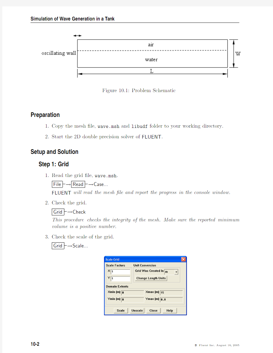
In this tutorial,we consider a rectangular tank with a length(L)of15m and width(W) of0.8m(Figure10.1).The left wall is assigned a motion with sinusoidal time variation.
The top wall is open to atmosphere and thus maintained at atmospheric pressure.The ?ow is assumed to be laminar.
Simulation of Wave Generation in a Tank
Figure10.1:Problem Schematic
Preparation
1.Copy the mesh?le,wave.msh and libudf folder to your working directory.
2.Start the2D double precision solver of FLUENT.
Setup and Solution
Step1:Grid
1.Read the grid?le,wave.msh.
File?→Read?→Case...
FLUENT will read the mesh?le and report the progress in the console window.
2.Check the grid.
Grid?→Check
This procedure checks the integrity of the mesh.Make sure the reported minimum
volume is a positive number.
3.Check the scale of the grid.
Grid?→Scale...
Simulation of Wave Generation in a Tank Check the domain extents to see if they correspond to the actual physical dimensions.
If not,the grid has to be scaled with proper units.
4.Display the grid(Figure10.2).
Display?→Grid...
(a)Click Colors....
The Grid Colors panel opens.
i.Under Options,enable Color by ID.
ii.Click Close.
(b)In the Grid Display panel,click Display
(c)Zoom in near the moving-wall(Figure10.3).
Simulation of Wave Generation in a Tank
Figure10.2:Grid Display
Figure10.3:Grid Display(Close-up of moving-wall)
Simulation of Wave Generation in a Tank
Step2:Models
1.Specify the solver settings.
De?ne?→Models?→Solver...
(a)Under Time,enable Unsteady
(b)Under Transient Controls,enable Non-Iterative Time Advancement.
(c)Click OK.
2.Enable VOF multiphase model.
De?ne?→Models?→Multiphase...
Simulation of Wave Generation in a Tank
(a)Under Model,enable Volume of Fluid.
The panel expands to show the other settings related to VOF model.Retain
the other settings as default.
(b)Click OK.
Step3:Materials
De?ne?→Materials...
1.Add liquid water to the list of?uid materials by copying it from the materials
database.
Simulation of Wave Generation in a Tank
(a)Click Fluent Database....
Fluent Database Materials panel opens.
Simulation of Wave Generation in a Tank
i.Select water-liquid(h2o
Scroll down to view water-liquid.
ii.Click Copy and close the panel.
(b)Click Change/Create and close the panel.
Step4:Phases
De?ne?→Phases...
1.Set air as primary phase and water as secondary phase.
(a)Under Phase,select phase-1.
The Type will be shown as primary-phase.
(b)Click Set....
i.Change Name to air.
ii.Select air in the Phase Material drop-down list.
iii.Click OK.
(c)Similarly,change the Name of phase-2to water and set its Type to water-liquid.
(d)Close the Phases panel.
Simulation of Wave Generation in a Tank
Step5:Operating Conditions
De?ne?→Operating Conditions...
1.Set the gravitational acceleration.
(a)Enable Gravity.
(b)Under Gravitational Acceleration,set Y to-9.81m/s2.
As the tank bottom is perpendicular to Y axis,gravity points in the negative
Y direction.
2.Set the operating density.
(a)Under Variable-Density Parameters,enable Speci?ed Operating Density.
(b)Retain the default density of1.225kg/m3.
Set the operating density to the density of the lighter phase.This excludes
the build-up of hydrostatic pressure within the lighter phase,improving the
round-o?accuracy for the momentum balance.
3.Set the reference pressure location.
(a)Under Reference Pressure Location,retain the default value of zero for both X
and Y.
This location corresponds to a region where the?uid will always be100%of
one of the phases(water).If it is not,it is recommended to change the region
to a appropriate location where the pressure value does not change much over
time.This condition is essential for smooth and rapid convergence.
4.Click OK to accept the settings and close the panel.
Simulation of Wave Generation in a Tank
Step6:Boundary Conditions
FLUENT maintains zero velocity condition on all the walls.Also,the pressure condition for outlet boundary at the top is set by default to zero gauge(or atmospheric).Hence, there is no need to change the boundary conditions.Retain all the boundary conditions as default.
Step7:UDF Library
De?ne?→User-De?ned?→Functions?→Compiled...
1.Click Load to load the UDF library.
The sinusoidal wall motion will be assigned using user de?ned function.A compiled
UDF library named libudf is created for this purpose.
Step8:Dynamic Mesh Model
1.Set the dynamic mesh parameters.
De?ne?→Dynamic Mesh?→Parameters...
Simulation of Wave Generation in a Tank
(a)Under Models,enable Dynamic Mesh.
The panel expands.
(b)Under Mesh Methods,disable Smoothing and enable Layering.
(c)Under the Layering tab,set Collapse Factor to0.4.
(d)Click OK.
2.Set the dynamic mesh zones.
De?ne?→Dynamic Mesh?→Zones...
(a)Under Zone Names,select moving-wall.
(b)Under Type,retain the default selection of Rigid Body.
(c)Under Meshing Options tab,set Cell Height to0.008m.
This is the average size of the cell normal to the moving wall.
(d)Click Create and close the panel.
Step9:Solution
1.Retain the default solution controls.
Solve?→Controls?→Solution...
Simulation of Wave Generation in a Tank
2.Initialize the?ow.
Solve?→Initialize?→Initialize...
(a)Click Init and close the panel.
The complete domain is now initialized with air.The water level required at
start(t=0)can be patched.
3.Create a register marking the region of initial water level.
Adapt?→Region...
Simulation of Wave Generation in a Tank
(a)Set X Max to be15m.
(b)Set Y Max to be0.5m.
(c)Click Mark and close the panel.
FLUENT displays the following message in the console:
8510cells marked for re?nement,0cells marked for coarsening.
4.Patch the initial water level.
Solve?→Initialize?→Patch...
(a)Under Registers to Patch,select hexahedron-r0.
(b)Under Phase,select water.
(c)Under Variable,select Volume Fraction.
(d)Set Value to1.
(e)Click Patch and close the panel.
Simulation of Wave Generation in a Tank
5.Display the zone motion to check the movement of moving-wall.
(a)Display the grid(Figure10.4).
Display?→Grid...
i.Under Surfaces,deselect default-interior.
Zoom-in the graphics window to get the view as shown in Figure10.4.
ii.Click Display.
Figure10.4:Grid Display Outline at t=0
(b)Display the zone motion.
Display?→Zone Motion...
Simulation of Wave Generation in a Tank
i.Under Motion History Integration,set Time Step to0.001.
ii.Set Number of Steps to300.
iii.Click Integrate.
iv.Under Preview Controls,set Time Step to0.001.
v.Set Number of Steps to300.
vi.Click Preview to observe the wall motion.
vii.Close the Zone Motion panel.
6.View the contours of volume fraction for water(Figure10.5).
Display?→Contours...
(a)Select Phases...and Volume Fraction in the Contours of drop-down lists.
(b)Under Phase,select water.
(c)Under Options,enable Filled.
(d)Click Display and close the panel.
Simulation of Wave Generation in a Tank
Figure10.5:Contours of Volume Fraction for Water
7.Enable the plotting of residuals during the calculation.
Solve?→Monitors?→Residuals...
(a)Under Options,enable Plot.
(b)Under Plotting,set Iterations to10.
This will display residuals for only the last10iterations.
(c)Click OK.
Simulation of Wave Generation in a Tank
8.Set hardcopy settings.
File?→Hardcopy...
(a)Under Format,select TIFF.
(b)Under Coloring,select Color.
(c)Click Apply.
(d)Click Preview.
The background of graphics window is changed to white.FLUENT will display
a question dialog box asking you whether to reset the window.
(e)Click Yes in the Question dialog box.
(f)Close the panel.
9.Set the commands to capture the images of contours.
You need to use Text User Interface(TUI)commands to achieve this.For most of the graphical commands,corresponding TUI commands are available.
Solve?→Execute Commands...
Simulation of Wave Generation in a Tank
(a)Set the number of De?ned Commands to3.
(b)Enable On option for all the commands.
(c)Under Every,set7for all the commands.
(d)Under When,set Time Step for all the commands.
(e)For command-1,specify the Command as:
display set-window1
This command will make the window-1active.
(f)For command-2,specify the Command as:
display contour water vof01
This command will display the contours of water volume fraction in the active
window.
(g)For command-1,specify the Command as:
display hard-copy"vof-%t.tif"
This command will save the image in the TIF format.
The%t option gets replaced with the time step number,when the image?le
is saved.The TIF?les saved can then be used to create a movie.For the
information on converting TIF?le to an animation?le,refer to
https://www.doczj.com/doc/bb4514366.html,/cfm/graphics01.htm
(h)Click OK to accept the settings and close the panel.
10.Set the surface monitors.
Solve?→Monitors?→Surface...
(a)Increase the number of Surface Monitors to1.
(b)Enable Plot for monitor-1.
(c)Under Every,select Time Step.
(d)Click on De?ne...next to monitor-1.
Simulation of Wave Generation in a Tank
(e)Select Area Weighted Average in the Report Type drop-down list.
(f)Select Grid and X-Coordinate in the Report of drop-down list.
(g)Under Surfaces,select moving-wall.
(h)Click OK to close both the panels.
11.Save the case and data?les(wave-init.cas.gz and wave-init.dat.gz).
File?→Write?→Case&Data...
Retain the default Write Binary Files option so that you can write a binary?le.The .gz extension will save zipped?les on both,Windows and UNIX platforms.
Simulation of Wave Generation in a Tank
12.Start the calculation.
Solve?→Iterate...
(a)Set the Time Step Size as0.001s
(b)Set Number of Time Steps to4000.
(c)Click Iterate.
Figure10.6:Scaled Residuals
13.Save the case and data?les(wave-4000.cas.gz and wave-4000.dat.gz).
二维模拟: 一、模拟类型: 1、 大区域空间速度场模拟 计算区域大小设置:迎风面是建筑长度的3倍,背风面是建筑长度的12倍,两侧面是建筑宽度的3倍,高度是建筑高度的4倍。 根据相似理论:l C -几何比例尺 速度比例尺:2 10l C C =υ 风量比例尺:2520l l Q C C C C =?=υ 热量比例尺: 250l T Q C C C Cq =?=? 2、 建筑户型温度场、速度场模拟 二、基本操作步骤及注意事项: A gambit 建模 1、 建模: 方法一:直接在GAMBIT 建模; 方法二:CAD 导入gambit ; 1) 在CAD 中用PL 线将户型的基本构造画出来,创建为面域; 2) 输入命令acisoutver ,把‘70’修改为‘30’。 3) “文件”——“输出”——sat 文件 4) 在gambit 中导入Acis 文件 注意:在用PL 线构画户型时,在进口和出口边界(窗户、内户门),要各边界端点连续画线。 2、 划分网格: Interval Size :50 3、 设置边界条件 内部开口边界(门)设置为internal ,房间相邻墙壁设置为Wall 4、 保存文件,并输出mesh 文件 B 导入fluent 计算: 1、 导入mesh 文件 2、 检查网格 3、 设置单位 gambit 里可以缩小建筑比例建模,在fluent 中设置单位恢复原模型。 4、 选择计算模型 5、 设置材料类型 6、 设置边界条件 7、 设置模拟控制条件 8、 边界初始化
9、设置监视窗口 10、设置迭代次数进行计算 11、结果显示 12、保存文件 三、需解决问题: 1、湍流强度等计算; 2、层流湍流界定问题; 3、壁面湿度设置问题; 四、待提高部分: 1、户型流场模拟时,墙壁考虑采用双钱; 2、南京理工校区原始模型(不简化)模拟; 3、三维模型模拟; 五、
实体入水模拟过程 3.2.1利用GAMBIT建立计算模型 1)启动GAMBIT,打开对话框如图3.2.1选择工作目录为D:\GAMBIT working。 图 3.2.1 2)首先建立等边三角形,单击Geometry Vertex Create Real Vertex,在Create Real Vertex面板的x、y、z坐标输入(0,0,0),单击Apply按钮生成第一个点,按同样的方法建立点(0.4,0,0)。然后单击Geometry Edge Create Straight Edge,在Create Straight Edge面板中选择点1与点2,连接这两点省成线段。如图3.2.2 图3.2.2 3)单击Edge面板中的Move/Copy Edges按钮,打开如图3.2.3的面板,选择线段1,单击copy按钮,并选择Operation为Rotate,在Angle栏输入60,其他保持默认,单击Apply 按钮。即旋转复制生成第二条线段。
图3.2.3 4)剩下的一条线段只需连接右侧两点即可,如图3.2.4所示。 图3.2.4 5)创建三角形面。单击Geometry Face Create Face from Wireframe,在Create Face from Wireframe面板中利用鼠标左键框选等边三角形的三条边,然后单击Apply按钮创建面。 6)由于三角形面域的位置不对,所以还要对其位置进行调整。首先需将其旋转210度。单击Face面板中的Move/Copy Faces按钮,在Move/Copy Faces面板中,选择面1(face.1),单击Move并选择Operation为Rotate,在Angle栏输入210,其他保持默认,单击Apply 按钮。其次,需要将三角形平移,在Move/Copy Edges面板中选择面1(face.1),单击Move 并选择Operation为Translate,在x与y栏分别输入3和8.4,单击Apply按钮完成平移操作,此时的视图窗口如图3.2.5所示。
Fluent数值模拟的主要步骤 使用Gambit划分网格的工作: 首先建立几何模型,再进行网格划分,最后定义边界条件。 Gambit中采用的单位是mm,Fluent默认的长度是m。 Fluent数值模拟的主要步骤: (1)根据具体问题选择2D或3D求解器进行数值模拟; (2)导入网格(File-Read-Case),然后选择由Gambit导出的msh文件。 (3)检查网格(Grid-Check),如果网格最小体积为负值,就要重新进行网格划分。(4)选择计算模型(Define-Models-Solver)。(6) (5)确定流体的物理性质(Define-Materials)。 (6)定义操作环境(Define-Operating Conditions)。 (7)指定边界条件(Define-Boundary Conditions )。 (8)求解方法的设置及其控制(Solve-Control-Solution)。 (9)流场初始化(Solve-Initialize)。 (10)打开残插图(Solve-Monitors-Residual)可动态显示残差,然后保存当前的Case和Data文件(File-Writer-Case&Data)。 (11)迭代求解(Solve-Iterate)。 (12)检查结果。 (13)保存结果(File-Writer-Case&Data),后处理等。 在运行Fluent软件包时,会经常遇到以下形式的文件: .jou文件:日志文档,可以编辑运行。 .dbs文件:Gambit工作文件,若想修改网格,可以打开这个文件进行再编辑。 .msh文件:Gambit输出的网格文件。 .cas文件:是.msh文件经过Fluent处理后得到的文件。 .dat文件:Fluent计算数据结果的数据文件。 三维定常速度场的计算实例操作步骤 对于三维管道的速度场的数值模拟,首先利用Gambit画出计算区域,并且对边界条件进行相应的指定,然后导出Mesh文件。接着,将Mesh文件导入到Fluent求解器中,再经过一些设置就得到形影的Case文件,再利用Fluent求解器进行求解。最后,可以将Fluent 求解的结果导入到Tecplot中,并对感兴趣的结果进行进一步的处理。
FLUENT 12 模拟步骤 Problem Setup 读入网格:file read case 选择网格文件(后缀为。Mesh) 1 General 1)Mesh(网格) > Check(点击查看网格的大致情况,如有无负体积等) Maximum volume (m3)(最大体积,不能为负) Minimum volume (m3)(最小体积,不能为负) Total volume (m3)(总体体积,不能为负) > Report Quality(点击报告网格质量) Maximum cell squish(最大单元压扁,如果该值等于1,表示得到了很坏的单元) Maximum cell skewness(最大单元扭曲,该值在0到1之间,0表示最好,1表示最坏) Maximum aspect ratio(最大长宽比,1表示最好) > Scale(点击缩放网格尺寸,FLUENT默认的单位是米) Mesh Was Create In(点选mm →点击Scale按钮且只能点击一次) View Length Unit In(点选mm →直接点击Close按钮不能再点击Scale按钮) > Display(点击显示网格设定)→弹出Mesh Colors窗口 Options(选Edges和Faces) Edge Type(点选All) Surface(点选曲面) →点击Display按钮 点击Colors按钮→弹出Mesh Display窗口 Options(点选Color by ID) →点击Close按钮→再点击Display按钮 2)Solver(求解器) > Pressure-Based(压力基,压力可变,用于低速不可压缩流动) > Density-Based(密度基,密度可变,用于高速可压缩流动) 3)Velocity Formulation(速度格式) > Absolute(绝对速度) > Relative(相对速度) 4)Time(时间) > Steady(稳态) > Transient(瞬态) 5)Units(点击设置变量单位) 点击按钮→弹出Set Units窗口→在Quantities项里点选pressure →在Units项里点选atm →点击
7.19多孔介质边界条件 多孔介质模型适用的范围非常广泛,包括填充床,过滤纸,多孔板,流量分配器,还有管群,管束系统。当使用这个模型的时候,多孔介质将运用于网格区域,流场中的压降将由输入的条件有关,见Section 7.19.2.同样也可以计算热传导,基于介质和流场热量守恒的假设,见Section 7.19.3. 通过一个薄膜后的已知速度/压力降低特性可以简化为一维多孔介质模型,简称为“多孔跳跃”。多孔跳跃模型被运用于一个面区域而不是网格区域,而且也可以代替完全多孔介质模型在任何可能的时候,因为它更加稳定而且能够很好地收敛。见Section 7.22. 7.19.1 多孔介质模型的限制和假设 多孔介质模型就是在定义为多孔介质的区域结合了一个根据经验假设为主的流动阻力。本质上,多孔介质模型仅仅是在动量方程上叠加了一个动量源项。这种情况下,以下模型方面的假设和限制就可以很容易得到: ?因为没有表示多孔介质区域的实际存在的体,所以fluent默认是计算基于连续性方程的虚假速度。做为一个做精确的选项,你可以适用fluent 中的真是速度,见section7.19.7。 ?多孔介质对湍流流场的影响,是近似的。 ?当在移动坐标系中使用多孔介质模型的时候,fluent既有相对坐标系也可以使用绝对坐标系,当激活相对速度阻力方程。这将得到更精确的源项。 相关信息见section7.19.5和7.19.6。 ?当需要定义比热容的时候,必须是常数。 7.19.2 多孔介质模型动量方程 多孔介质模型的动量方程是在标准动量方程的后面加上动量方程源项。源项包含两个部分:粘性损失项(达西公式项,方程7.19-1右边第一项),和惯性损失项(方程7.19-1右边第二项) (7.19-1)
空调间内空气流场的模拟 模拟课题名称:空调间内空气流场的模拟 模拟的步骤: 1:gambit建立空间模型及建立网格 1.1打开gambit,选择文件的存储路径。 为了寻找的方便,我们将文件尊放在d盘fluent文件下 点击run,进入gambit界面; 1.2建立空调间的空间模型 点击体控制面板中的体控制按钮直接生成六面体,选择direction为+x+y+z方向输入房间尺寸,生成房间如图
同样的方法生成空调的六面体,并将六面体通过移动的选项将六面体移动到正确的位置上如图: 因为整个的计算区域为空调间减去空调的空间所以选择选项,将空调的空间去除,经过渲染之后得到下图: 这样计算区域的几何模型就建立起来了。 1.3网格的划分
这里我们直接对体进行网格划分点击,进入网格划分界面,选择该体,采用六面体的网格单元和submap网格划分方法进行划分如图 Interval size输入0.05,建立网格如图 如图,我们可以看到总共建立了359840个网格。接下来需要对网格单元记性检 查,经过检查发现网格符合要求。 1.4定义边界类型
本文定义房间的上下左右先后分别为壁面边界,空调的下边界为速度进口,空调的上边界为速度出口空调的其他面为壁面边界。建立的过程如图 建立完成后得到:
1.5保存文件后安全退出 执行File Export Mash,输出三维的数据文件,不要在2维的地方打勾,为 了以后查找的方便我们将文件的名字改为kongtiaojian,最后执行Exit安全退出。这里注意不要点右上角的,要选择exit键才能安全退出,否则生成的是 碎片文件。 2 fluent模拟 2.1文件的读取和检查 打开fluent三维单精度计算器如图,执行Flie Read Case,读入我们已经划分好的网格文件,当出现 表示网格文件读入完毕。执行Grid Check 检查网格,表示网格检查完毕。执行Grid Scale我们可
一收缩-扩张喷管实例1.1问题描述 本节内容主要依托收缩-扩张喷管内的流动计算展开。喷管外形如图1-1所示,A 为沿轴圆形截面面积,喷管的外形尺寸满足如下条件(单位:m): 21.0x A +=5 .05.0<<-x 计算求解时可以将模型琪简化为二维轴对称问题,边界条件为:入口压力P m =101325Pa,入口总温T i0=300K,出口静压P 0=3738.9Pa。 图1-1喷管几何示意图 1.2创建几何模型 (1)设定工作目录 File→Change Working Dir,选择文件存储路径。 (2)创建Point,如图1-2所示。 Step 1通过输入坐标的方法创建P_1、P_2。选择Geometry 标签栏中的,单击,选择Create 1point(创建一个点),输入P_1的坐标,单击Apply 按钮确定,如图1-3所示。P_2创建方法与之相似,坐标为(0.5,0,0)。 Step 2创建点集3。因为横截面积为21.0x A +=,因此沿X 轴方向半径的函数为:5.02]/)1.0[()( x x R +=。单击,在Explicit Locations 下拉菜单中选择Create Multiple points,按照如图1-4所示输入数据,单击Apply 按钮确定。单击Apply 按钮确定。
图1-3创建P_1图1-4创建点集3 (3)创建Curve,如图1-5所示。 图1-5创建Curve结果图 Step1选择Geometry标签栏,单击创建Curve。如图1-6所示,单击,再单击,依次选择点集3中的各点连成曲线,创建C_4。 Step2采用Step1的方法创建其余三条Curve。 (4)定义Part。 ICEM中定义Part的名称将会是导出网格后边界的名称,可以简化在求解器