
Self-Calibration of a Light Striping System by Matching Multiple3-D Pro?le Maps
Olli Jokinen
Institute of Photogrammetry and Remote Sensing
Helsinki University of Technology
P.O.Box1200,FIN-02015HUT,Finland
E-mail:Olli.Jokinen@hut.fi
Abstract
A new method is proposed for re?ning the calibration of a light striping system including a projective transforma-tion between the image plane of the camera and the plane of the laser sheet,and also the direction of the scanning with respect to the plane of the laser sheet.The re?nement is ob-tained through weighted least squares matching of multiple pro?le maps acquired from different viewpoints and regis-tered previously using an approximate calibration.
Testing with synthetically generated pro?le maps shows that if the geometry of the object is appropriate and the registration parameters and the intrinsic parameters of the system are known exactly,then a calibration accuracy of
%relative to the scene dimensions can be achieved as the average noise level in the maps used for the calibration decreases from down to zero pixels.It is also possible to adjust several calibrations at the same time. The registration and calibration parameters can be re?ned simultaneously,but a close initial estimate and rather com-plex object geometry are needed for an accuracy of% when the average noise level is pixels.Determining the corresponding points by interpolation on the paramet-ric domains of the maps yields higher accuracy than per-pendicular projection to the tangent planes at the closest points in3-D in both registration and calibration tasks.The highest accuracy is achieved when the interpolation errors are as equal as possible within the overlapping areas.
1.Introduction
Light striping is a well-known technique for digitizing object surfaces.It is based on projecting a stripe of laser light on the surface and viewing it by a CCD camera.Scan-ning multiple pro?les by moving the object stepwise into a ?xed direction yields a set of3-D points that may be rep-resented as a pro?le map[7].Calibration of the system in-cludes solving the relative orientation between the camera and laser given by a projective transformation between the image and laser planes,and solving the direction of the ob-ject movement with respect to the plane of the laser sheet. In this paper,we assume that the intrinsic parameters of the camera and laser have been determined in advance.
Most previous approaches for the calibration use a sep-arate calibration target with known dimensions.In[15], an arrangement of orthogonal planes whose equations are known accurately in world coordinates and a set of detected world plane to image point correspondences are used to es-timate the parameters of the projective transformation.In [19],they use four edge points of a calibration object having an extrusion axis perpendicular to which all the cross sec-tions are the same.The case where the laser sheet is not per-pendicular to the direction of the object movement thus al-lowing a more?exible scanning of complex objects is stud-ied in[4].They propose an on-line calibration method using the vertices of a tetrahedron target for?nding the transfor-mation between a non-Cartesian skewed sensor frame and a Cartesian object frame.In[9],errors in scale and axes’non-orthogonality are reduced by a self-calibration method based on measuring a scene of balls on a plate from dif-ferent viewpoints.A reference object is also used in[17]. The accuracy reported after calibration is typically%of the depths measured[15]or%of the?eld of view[18].
In this paper,we present a new method for the calibra-tion of the light striping system.An initial calibration ob-tained using a pre-measured target is re?ned by an area-based matching of multiple3-D pro?le maps acquired from different viewpoints and registered previously to the same coordinate system.We thus derive the3-D structure of the object from shape correspondences.Consequently,our self-calibration method can be viewed as an extention to solving the structure from motion problem,where only point or fea-ture correspondences in a sequence of images(acquired us-ing either a calibrated or non-calibrated camera)have been
considered previously,see e.g.[1,2,10,14,21,23,24].
The calibration result given by our algorithm evidently depends on the accuracy of the registration.On the other hand,an accurate calibration is important for the registra-tion as systematic errors in the data may lead to a biased registration estimate.As studied in[13],the shape of the measured surface may be clearly deformed if there are er-rors in the calibration points used to estimate the parameters of the projective transformation.In this paper,we test how much the registration errors affect the calibration result and vice versa.We investigate solving the registration and cal-ibration parameters either sequentially or simultaneously. We also compare our parametric method to determine the corresponding points in the,hereby named,iterative para-metric point(IPP)algorithm[7]to the well-known iterative closest point(ICP)algorithm[3].
The paper is organized as follows.In the following sec-tion,we describe the measuring system and present the method for its calibration.We consider?rst a pure calibra-tion task and discuss then various extensions to the method related to the number of unknown calibration parameters and to solving both registration and calibration.A thorough testing of the different cases is performed in Section3and the conclusions are summarized in Section4.
2.Calibration method
In this section,we present an area-based method for the self-calibration of the light striping system.
2.1.System description and the unknown parame-
ters
The light striping system is illustrated in Fig. 1.The right-handed rectangular laser coordinate system is ?xed so that the-plane is parallel to the plane of the laser sheet and the?rst pro?le measured has the value. The object is moved in the direction of the negative-axis of a skewed coordinate system de?ned so that the and axes coincide with the and axes,respectively. The coordinates of the image of the camera are denoted by and while stands for the pro?le index.We use every th row(is a nonnegative power of two)and all columns of the image and the coordinates ,where and,de?ne a pro?le map coordinate system.We have where the coef?cients determine the projective transformation between the image plane and the plane of the laser sheet,and de?nes the step size of the object movement.The skewed frame is recti?ed by
by measuring the image coordinates of four corner points
of an object of known geometry.The parameters and are usually near zero.
The matching algorithm is a re?ned version of the itera-
tive parametric point(IPP)algorithm we have developed in [7]for solving the registration problem.It iterates two steps
until convergence namely the corresponding points are de-termined according to the current calibration and the cali-
bration parameters are updated so that the weighted mean
squared distance between the corresponding points is min-imized.The corresponding points between and are
de?ned on as described in[7].The distance is given by
,where is an image on whose values equal the transformed observations of in the pro?le map
coordinate system of according to the current calibration and known registration parameters,and is an image on
whose values are the interpolated values of at the interme-
diate locations hit by the transformed image .The bilinear interpolation has been replaced almost ev-
erywhere by a bicubic one which uses the values in the
neighborhood around to interpolate?rst in one direction and then in the other direction by a polynomial of third de-gree.In case there are not enough data around for the bicubic interpolation,we use the bilinear one.The inter-polation errors are smaller in the bicubic one especially for curved surfaces.They depend also on the geometry of the object surface and are usually not the same over the whole view.Consequently,the interpolation errors may cause a systematic error to the calibration result.
The weighted mean squared distance to be minimized in
calibration is given by
(3)
where are the weighting images between the corre-sponding points,,’’denotes the dot product of images,and is a unit image on having ones at all locations.Within the overlapping ar-eas,the weighting images adaptively reject incompatible matches in regard to the statistical distribution of the dif-ference in the direction of the surface normal and the statis-tical distribution of the distance between the corresponding points[7,22].The weighting near edges has been re?ned so that the correspondence is given zero weight if at least one of the corresponding points is near an edge.The edges are located in areas where the Laplacian does not change smoothly.A pixel location is near an edge if the value of the Laplacian image at the location differs from the mean value in the neighborhood of the location more than a threshold. Note that setting only a threshold for the Laplacian does not work for curved surfaces.We remove the edge locations and match the views only on smooth surfaces,since large in-terpolation errors near edges disturb correcting small shape deformations of the whole data which result from the er-rors in the calibration parameters.We have also introduced
a new weighting image that takes into consideration the precision of the data.The value of this image at equals v Var,where the variance is es-timated using the rules of the?rst order error propagation
and the scale is selected according to the noise level of the data so that the weights are around one.
The Levenberg-Marquardt algorithm is used to update the calibration parameters.The processing is sped up matching the surfaces hierarchically.Moreover,we have changed the normal estimation from the eigenvector estima-tion in a neighborhood to the one based on estimating the tangent vectors of two curves on the surface.For, we use the parabolas through three points along the and axes,respectively,and for,the same polynomials as in interpolation.The method can be vectorized and it per-forms about42times faster than our previous non-parallel estimation.The speed-up is important since the surface nor-mal changes each time the calibration parameters are up-dated.The iteration is stopped when the merit function is smaller than,or when the merit function previously decreased relatively less than0.1per cent,or when all the parameters changed relatively less than0.01per cent,or when the number of iterations exceeds100.The iteration is not terminated,however,if the merit function increased previously and the number of iterations is less than105. 2.3.Extensions to the basic problem
In the previous subsection,we considered the pure cal-ibration task and assumed that the registration parameters are known.This is not usually the case in practice.The pro-?le maps may also have been measured at different times with different calibration parameters if one wants,e.g.,to measure previously occluded parts of the object after hav-ing analyzed the data acquired by then.We consider the following extensions to the pure calibration.
The registration and calibration algorithms are iterated several times.All the maps are assumed to have the same calibration parameters.
The registration and calibration parameters are solved simultaneously.All the maps are assumed to have the same calibration parameters.
All the maps do not have the same calibration param-eters.The unknown parameters are given in a vector
,where.The registra-tion parameters are assumed known.
In all these cases,in Eq.(3)is minimized but the un-known parameters vary,being either,or,or,or and .Whether the algorithm converges to a correct solution
or not depends evidently on such things as the complexity
of the scene and the number of the maps in regard to the
number of the parameters to be solved.
3.Testing
In this section,we show the results of testing the pro-
posed self-calibration method and the extended problems
with synthetic data and one example with real data.The al-
gorithms have been implemented using the MATLAB soft-
ware[11].The computations have been performed in a Dig-
ital Personal Workstation433au and the largest cases requir-
ing much memory in a SGI Origin2000hardware.
3.1.Generating synthetic data
The?rst synthetic object considered consist of a box,
a cone,an elliptic paraboloid,and a planar background
the equations of which are given in an object coordinate
system.The transformation from the object to
the laser coordinate system de?nes the scanning
path as,where
is the starting point in the object coordinates and
pixels,where is the coor-
dinate of the unit surface normal in the laser frame and
is the number of scans.This noise model is based on our ex-
perience that the deviation depends somehow on the width
of the stripe projected onto the object surface[8].
3.2.Testing the basic problem
The calibration algorithm has been tested in several cases
by performing20trials for each test.In each trial,the true
calibration parameters are altered by adding normally dis-
tributed noise with zero mean and deviation to the im-
age coordinates of the four known corresponding points be-
tween the laser and image planes and with zero mean and
deviation to the parameters and.The noise
added to the data is changed each time,too.A single trial
is considered successful if the mean of the relative errors
(MRE)in the calibration parameters given by the trial is
less than5%.The estimated calibration is given by the
average over successful trials.The accuracy of the method
is evaluated by two?gures.The?rst one is the MRE in the
estimated parameters and the second one is the root mean
squared error(RMSE)in relative to the scene dimension
,i.e.,the root of the squared distance between the true data point in the frame and the one obtained using the estimated calibration divided by the squared scene di-mension for the row of the image the observation was made and averaged over all data points in successful trials.Table 1gives an idea of how much the perturbation of the four image coordinates and parameters and affects these error measures.The?gures in Table1have been calculated as a mean of100initial calibrations for each.
Table1.Relative errors when the initial cali-
bration is used,typically.
0.1
60.22
0.3
110.42
0.5
29 1.2
1.5
84 2.7
3.0
24062
5.0
succ.%MRE()%RMSE()%
1000.0130.0030
0.2
1000.0110.0033
0.4
1000.0130.0038
1.0
950.0130.0035
2.0
950.0130.0027
4.0
600.0140.0026
In the?rst experiment,it was tested how close the ini-tial calibration should be so that the algorithm converged to a correct solution.Four pro?le maps were generated from different viewpoints over the synthetic object and220tri-als were performed for11different values of(20trials for each,).The percentages of successful cal-ibrations are shown in Table2.We see that100%conver-gence is obtained for and the method performs well for.The accuracy of the method is high,about
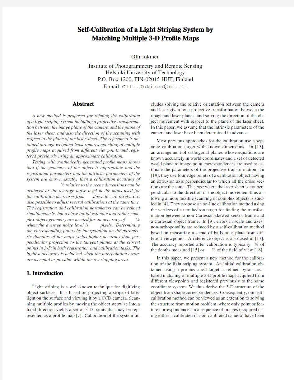
Figure3.Weighted distances d
within the overlapping area a)before and b)
after matching.
1:30,000relative to the scene dimension on the average for successful trials.The errors in,,and were also computed and it was found that the errors in are an order of magnitude smaller than in and.Figure3further il-lustrates the weighted distances between the corresponding points of the?rst map and the fourth one.Figure3a is ac-cording to an initial calibration generated with and leading to a successful trial while Figure3b is according to the estimated from all the successful trials with
and further re?ned by performing some more iterations.We see that the systematic differences of the order of several pixels have been eliminated down to the noise level of the data.The data sets have been plotted according to the re-?ned calibration in the reference frame in Fig.4.
The algorithm was tested next for different noise lev-
Figure4.Data sets in the reference frame after
calibration.
els in the data.The same four maps were used as above and the tests were performed for two values of.The re-sults are shown in Table3and we see that it is somewhat
more likely to obtain a correct solution if the noise level is higher,i.e.,is smaller.The accuracy increases up
till when the noise level decreases.This is since shape deformations can be better distinguished and thus corrected during calibration if the noise level is lower.
In case,there are only interpolation errors left and their contribution to the calibration result is very min-imal if the initial calibration is close.If the bilinear in-
terpolation was used,we obtained MRE% and RMSE%for noise-free data.The bicubic one is better since the interpolation errors are more evenly distributed within the overlapping areas for the dif-ferent types of surfaces we are having in the data sets.On the average,the noise added to the pro?le maps results in an error in of%relative to the scene dimension for,respec-tively.The systematic errors caused by the errors in the calibration are thus of the same order of magnitude as the noise in this and the previous experiment.
The testing was carried on using three pro?le maps gen-erated from different viewpoints over one corner of the box and the background plane so that there were only data from four planes in each of the maps.The same tests were per-formed as above and the results are given in Tables4and 5.When compared to Tables1and2,we see that the per-centages of successful calibrations are roughly similar but the accuracy is lower than in the case of four maps over the whole object.The method works,however,although the geometry of the object is simple.We tested also using only Table3.Calibration results for different noise levels in the data when and
().
1
1000.0130.0030
100
1000.000910.00035
1
1000.00790.0034
100
650.00130.00058
succ.%MRE()%RMSE()%
1000.470.021
0.5
1000.400.023
1.5
850.370.015
3.0
800.170.014
5.0
Table5.Calibration results for different noise levels in the data(one corner of the box,
).
1
1000.470.021 100
1000.0790.0019
succ.%MRE()%RMSE()%
1000.0330.0021
3
1000.00390.0024
5
1000.00170.00034
7
0.010.10.5 1.0
0.24 4.61041
RMSE()%
0.010.10.5 1.0
0.0160.290.58 6.3 parameters.Good results were obtained with an object con-sisting of72planar patches in different orientations.This
object was generated triangulating a set of randomly per-
turbed3-D points.A pro?le map over the object is shown in Fig.5.Another object appropriate for the simultaneous
registration and calibration might be the registration aid de-signed in[12].
Figure5.A pro?le map over the triangulated
mesh.
The results of the simultaneous registration and calibra-
tion using the object in Fig.5are shown in Tables9and
10.The method gives100%success only if the initial esti-mates are close to the true ones.For,,and ,an accuracy of relative to the scene dimension can be obtained.For these values,the
MRE in the initial parameters was2.7times larger than in
the solution on the average.The error in includes the registration error when transforming the other data sets to the?rst frame.For comparison,the case of four maps was
also solved sequentially.The registration was kept?xed
when the calibration was re?ned and vice versa.The results in Table11show that the estimates get slowly better as more iterations are performed,but the accuracy of the calibration is an order of magnitude lower than in the simultaneous so-lution.In view of Tables7and8,it is our experience that further iterations do not essentially improve the results.
Table9.Simultaneous registration and cali-
bration as a function of the noise levels in the initial estimates().
,
succ.%
0.060 1.00.970.47
MRE()%
0.0270.430.490.072
Table10.Simultaneous registration and cali-
bration as a function of the number of maps ().
succ.%
0.250.0600.120.40
MRE()%
0.0630.0270.0470.089
Table11.Sequential registration and calibra-tion().
iteration
succ.reg.%
0.290.320.270.26
succ.cal.%
1.10.850.810.76
Some experiments were also performed where two or three sets of calibration parameters(,,and)were solved simultaneously using four or six maps.The registra-tion parameters were given the true values.For comparison, each was solved separately using the same two or three maps that were used in the simultaneous case.The results are shown in Table12.In the?rst case of four maps,solv-ing separately did not succeed while solving it together with gave accurate results.The simultaneous solutions are more accurate than the separate ones in the other cases, too.Table12.Calibration results for(
).
simultaneously
100100100 MRE()%
0.00410.00290.0021
succ.%
1.10.0280.25 RMSE()%
IPP
succ.%MRE()%RMSE()%
1000.330.035
10
1000.0270.0046 1000
700.330.071
ICP
succ.%MRE()%RMSE()%
0--
10
10 2.10.21 1000
55 2.50.28
Table14.Percentages of successful registra-tions for three methods().
IPP,Lev.-Marq.
1001009090
ICP,unit quat.
0.5 1.0 1.5 2.0
0.00180.00120.260.00088 IPP,unit quat.
0.250.470.69 1.0
In order to complement our previous work in[7,8],we compared the IPP and ICP algorithms for the pure regis-tration task,too.Only two maps were used so that the method of unit quaternions could be applied to update the registration parameters in the ICP algorithm.A third dis-tance image was also implemented where the correspon-dences were established by the parametric method,but the distance was measured in the frame and the reg-istration parameters were updated using the method of unit quaternions.The registration results for the three methods are shown in Tables14and15.We may realize that the IPP algorithm combined with the Levenberg-Marquardt method works best and gives the highest accuracy.More studies on the convergence range of the ICP algorithm can be found in[6].The closed form solutions to updating the registra-tion parameters between two data sets including the meth-ods based on the singular value decomposition,orthonormal matrices,unit quaternions,and dual quaternions are com-pared in terms of the accuracy,robustness,stability,and computing time in[5].
3.5.Testing with real data
The real data case consists of four pro?le maps over a scale model of an urban area.The maps were scanned with the same calibration from slightly different viewpoints so that the overlapping areas were large.The data sets were registered?rst sequentially and then simultaneously using the IPP algorithm.The initial calibration given by four points was then re?ned by the IPP calibration method with ?xed registration.Finally,the maps were matched with both the registration and calibration parameters as unknowns. The weighting based on the precision of the data was not used since only single scans were available.The maps con-tain much edge locations and it worked better to weight them with a decay function rather than to give zero weight. The matched data sets have been plotted in the reference frame in Fig. 6.Figure7shows the magni?cation of a building in the lower right corner of Fig.6.There are some errors left after registering and these have been corrected during the calibration.The simultaneous registration and calibration does not bring much visual improvement in this case.The pro?le maps were measured with a non-calibrated camera so that the assumption on a projective transforma-tion between the image and laser coordinates does not nec-essarily hold
here.
Figure6.Matched data sets in the reference
frame after simultaneous registration and cal-
ibration.
4.Discussion and the concluding remarks
In this paper,we have presented a novel method for the self-calibration of the light striping system based on match-ing multiple pro?le maps acquired from different view-points.The core of the method is the iterative paramet-ric point algorithm developed previously for the registration task and re?ned now for the calibration case.
A thorough testing with synthetic data proved the high accuracy and precision of the method if the registration pa-rameters and the intrinsic parameters of the system were as-sumed known.After calibration,we reported the RMS error in relative to the scene dimension of
depending on the noise level in the maps used for the cal-ibration.If the registration was also unknown,the best re-sults were obtained when the registration and calibration pa-rameters were re?ned simultaneously while the sequential approach proved to be unsuitable.The simultaneous solu-tion required,however,that the initial estimate was closer
to the true one and the object geometry was more com-plex than in the pure calibration task with known registra-tion.In the simultaneous case,we obtained an accuracy of
for a moderate noise level in the data with an object consisting of72planar patches in different orientations.These?gures are due to errors in the calibra-tion and the actual measuring accuracy of the system de-pends much on how accurately the stripe can be measured from the image.
In order to achieve the high calibration accuracy,we de-termined the corresponding points on the parametric do-mains of the maps,included the precision of the data in the weighting,performed the matching only on smooth areas, and used the bicubic interpolation so that the interpolation errors were as equal as possible within the overlapping ar-eas.Since edge areas may contain useful data for the match-ing,another possibility instead of removing them might be to estimate the magnitude of the interpolation errors us-ing higher order derivatives and weight the corresponding points accordingly.The interpolation errors could also be reduced increasing the density of pro?les and image obser-vations in critical areas.
The testing further showed that a rather close initial cal-ibration was needed in all cases for a successful conver-gence.It was also possible to re?ne several calibrations simultaneously.The number of maps did not have to be large if the geometry of the object was appropriate within the overlapping areas.A comparison indicated the superi-ority of our IPP algorithm to the standard ICP algorithm. An example with real data showed the qualitative improve-ment of the matching due to re?ning the calibration.The techniques presented for generating synthetic pro?le maps may also be utilized in other applications such as planning convenient scanning paths for object digitization if,e.g.,a CAD model of the object is available.
Acknowledgments
We would like to thank Henrik Haggr′e n for several dis-cussions on calibration.
References
[1]S.Abraham and W.F¨o rstner,“Calibration errors in
structure from motion,”Proc.DAGM Symposium Mus-tererkennung,pp.117-124,Stuttgart,1998.
[2]P.A.Beardsley, A.Zisserman,and D.W.Murray,
“Sequential updating of projective and af?ne structure from motion,”International Journal of Computer Vi-sion,V ol.23,No.3,pp.235-259,1997.
[3]P.J.Besl and N.D.McKay,“A method for registration
of3-D shapes,”IEEE Transactions on Pattern Analysis
and Machine Intelligence,V ol.14,No.2,pp.239-256, 1992.
[4]C.Che and J.Ni,“Modeling and calibration of a
structured-light optical CMM via skewed frame repre-sentation,”Journal of Manufacturing Science and En-gineering,Transactions of the ASME,V ol.118,No.4, pp.595-603,1996.
[5]D.Eggert,A.Lorusso,and R.B.Fisher,“Estimating
3-D rigid body transformations:A comparison of four major algorithms,”Machine Vision and Applications, V ol.9,No.5/6,pp.272-290,1997.
[6]H.H¨u gli and C.Sch¨u tz,“Geometric matching of3D
objects:assessing the range of successful initial con-?gurations,”Proc.International Conference on Recent Advances in3-D Digital Imaging and Modeling,pp.
101-106,Ottawa,1997.
[7]O.Jokinen,“Area-based matching for simultaneous
registration of multiple3-D pro?le maps,”Computer Vision and Image Understanding,V ol.71,No.3,pp.
431-447,1998.
[8]O.Jokinen and H.Haggr′e n,“Statistical analysis of two
3-D registration and modeling strategies,”ISPRS Jour-nal of Photogrammetry and Remote Sensing,V ol.53, No.6,pp.320-341,1998.
[9]J.P.Kruth,P.Vanherck,and L.De Jonge,“Self-
calibration method and software error correction for three-dimensional coordinate measuring machines us-ing artifact measurements,”Measurement,V ol.14,No.
2,pp.157-167,1994.
[10]Q.-T.Luong and O.D.Faugeras,“Self-calibration of
a moving camera from point correspondences and fun-
damental matrices,”International Journal of Computer Vision,V ol.22,No.3,pp.261-289,1997.
[11]MATLAB User’s Guide,The MathWorks,Inc.,1992.
[12]R.Pito,“A registration aid,”Proc.International Con-
ference on Recent Advances in3-D Digital Imaging and Modeling,pp.85-92,Ottawa,1997.
[13]P.P¨o ntinen,Kolmiulotteinen videodigitointi(Three
Dimensional Video Digitizing),Master’s thesis, Helsinki University of Technology,1994(in Finnish).
[14]R.V.Raja Kumar,A.Tirumalai,and R.C.Jain,“A
non-linear optimization algorithm for the estimation of structure and motion parameters,”Proc.IEEE Com-puter Society Conference on Computer Vision and Pat-tern Recognition,pp.136-143,Rosemont,IL,1989.
[15]I.D.Reid,“Projective calibration of a laser-stripe
range?nder,”Image and Vision Computing,V ol.14,
No.9,pp.659-666,1996.
[16]G.X.Ritter,J.N.Wilson,and J.L.Davidson,“Image
algebra:an overview,”Computer Vision,Graphics,and
Image Processing,V ol.49,pp.297-331,1990.
[17]J.R¨o ning,A.Korzun,and J.P.Riekki,“Extrinsic cali-
bration of single-scanline range sensor,”Industrial Op-
tical Sensors for Metrology and Inspection,Proc.SPIE
2349,pp.35-43,Boston,1994.
[18]G.Sansoni,S.Corini,https://www.doczj.com/doc/d817615228.html,zzari,R.Rodella,and F.
Docchio,“Three-dimensional imaging based on Gray-
code light projection:characterization of the measuring
algorithm and development of a measuring system for
industrial applications,”Applied Optics,V ol.36,No.
19,pp.4463-4472,1997.
[19]A.Sommerfelt and T.Melen,“A simple method for
calibrating sheet of light triangulation systems,”Opti-
cal3-D Measurement Techniques III:Applications in
inspection,quality control and robotics,A.Gruen and
H.Kahmen(Eds.),pp.414-423,Herbert Wichmann
Verlag,Karlsruhe,1995.
[20]E.Trucco,R.B.Fisher,A.W.Fitzgibbon,and D.
K.Naidu,“Calibration,data consistency and acquisi-
tion with laser stripers model,”International Journal of
Computer Integrated Manufacturing,V ol.11,No.4.,
pp.293-310,1998.
[21]J.Weng,N.Ahuja,and T.S.Huang,“Optimal motion
and structure estimation,”IEEE Transactions on Pat-
tern Analysis and Machine Intelligence,V ol.15,No.9,
pp.864-884,1993.
[22]Z.Zhang,“Iterative point matching for registration of
free-form curves and surfaces,”International Journal
of Computer Vision,V ol.13,No.2,pp.119-152,1994.
[23]Z.Zhang,“Estimating motion and structure from cor-
respondences of line segments between two perspective
images,”IEEE Transactions on Pattern Analysis and
Machine Intelligence,V ol.17,No.12,pp.1129-1139,
1995.
[24]Z.Zhang,“Motion and structure of four points from
one motion of a stereo rig with unknown extrinsic pa-
rameters,”IEEE Transactions on Pattern Analysis and
Machine Intelligence,V ol.17,No.12,pp.1222-1227,
1995.Figure7.Magni?cation of a building after a)
registration,b)calibration,c)simultaneous
registration and calibration.
中国宏观经济形势的分析与预测 宏观经济形势分析以及未来发展趋势的判断是一个重要而复杂的课题,不仅需要运用科学性、技术性高的方法,还应该遵循正确的原则;既要重视宏观经济的微观基础,又要考虑宏观经济的基本面,对国内外因素及其影响进行全面的分析,从而提高我国宏观经济形势分析的科学性以及对未来发展趋势判断的准确性,促进我国经济更快更稳的发展。 标签:宏观经济形势经济分析未来发展趋势 1 概述 对我国宏观经济形势的分析及未来经济形势的判断影响着政府、企业或个人对市场的决策和调控的决策。在实际分析和判断中,如果忽视了正确的原则可能造成宏观经济判断上的分歧,使得宏观经济形势的分析与判断的盲目性和随意性,难以确保我国经济健康、可持续发展。因此相关部门必须科学合理的分析与判断我国宏观经济形势,准确的把握未来经济发展趋势,从而提高个人和企业的经济效益,促进政府部门经济调控的有效性。 2 我国宏观经济形势分析情况 2.1 中国经济发展的优势与机遇一是我国经济顺利驶入了稳定发展的正常航道;二是内生性增长机制起到了重要的作用;三是中国出口呈现出了恢复性增长的趋势。 另外,目前中等收入国家向逐步向高收入国家迈进,内需潜力巨大;工业化、信息化、农业现代化具有较大的发展空间;企业在面临市场经济改革或者调控时,自我发展能力和适应能力逐渐增强;国民储蓄率较高,对宏观经济政策发展空间较大等。 2.2 中国经济发展存在的问题与矛盾首先是不平衡、不协调、不可持续的问题没有得到根本的解决,我国通胀压力有增强的趋势不利于市场调控,使得我国房地产行业和汽车行业无法形成新的增长点,房价、物价持续上涨。另外地方债务风险、局部金融风险仍然存在并在积累,诸多中小型企业发展遇到了资金短缺的问题,出现一方面贷款宽松,一方面贷款难的问题同时存在,给货币政策宏观调控带来了巨大的阻力。 3 中国宏观经济形势分析及未来趋势判断需要把握的问题 3.1 确定经济变量合理的参照对我国宏观经济形势的分析以及未来趋势的判断,涉及到的宏观经济变量范围较广,往往需要正确的确定相关参照值,参照值可以是正常值、过去值或者目标值,往往需要根据实际的经济变量,以确定不同意义的参照值。就GDP增长率来讲,其主要反映的是宏观经济运行态势的一
中国宏观经济形势分析 当前中国经济正处在由企稳回升走向全面恢复的关键阶段,应努力保持来之不易的经济成果,妥善处理经济运行中的突出矛盾与困难,为下一阶段经济平稳运行打好基础。宏观调控应根据新形势新情况不断提高政策的针对性和灵活性,把握好政策实施的力度、节奏和重点。 一、国民经济全面恢复物价上涨压力加大 1.消费增长保持稳定 (1)推动消费增长的主要因素:一是政策因素将继续成为支持消费增长的重要动力。扩大消费需求,提高消费对经济增长的贡献度是当前及未来一段时间我国宏观调控政策的重点,二季度家电、汽车、节能产品消费政策将继续完善,增加城乡居民特别是低收入者收入的措施将进一步落实,“万村千乡”和“双百”工程建设将深入推进,政策对消费的推动作用依然较强。二是城乡居民收入增长将提高社会消费意愿。一季度,农村居民人均现金收入实际同比增长9.2%,比上年同期加快0.6个百分点;城镇居民人均可支配收入实际同比增长7.5%。根据一季度人民银行储户问卷调查,城镇居民判断收入增加的占比从2009年二季度的12.6%回升到2010年一季度的21.3%,实际收入与收入预期的改善将提高居民消费能力与意愿。三是世博会召开刺激消费增长。二季度世博会在上海举行,届时周边地区旅游、会展等生活性与生产性服务消费将大幅增加。四是居民消费价格上涨,将促使消费名义增速走高。2009年二季度CPI同比负增长1.3%,而今年二季度CPI呈明显上行趋势,社会消费品零售总额名义增速将提高。 (2)抑制消费增长的主要因素:一是国家近期连续出台的房地产调控政策效果在二季度显现,与住房相关的家具、建材消费增长将趋缓。而且,前期房价涨幅过大,对已买房居民下一阶段的其他消费形成一定制约。二是干旱、地震等自然灾害将减少当地居民收入,降低居民生活水平,导致局部地区消费能力下降。三是近期粮食、蔬菜、水果价格涨幅较高,成品油价格调整,不利于居民实际购买能力提高。 总体而言,消费需求将保持稳定,初步预计,二季度社会消费品零售总额名义增长19%。 2.物价上涨压力加大 一是翘尾因素提高二季度物价涨幅。经计算,二季度CPI翘尾因素为1.6个百分点,PPI为4.4个百分点,分别处于全年翘尾值次高和最高水平,即使不考虑新涨价因素,二季度CPI与PPI也将呈现一定幅度上升。二是输入型物价上涨动力增强。世界经济复苏导致国际大宗商品价格暴涨,国
1、SDN是什么? SDN(Software Defined Network)即软件定义网络,是一种网络设计理念。网络硬件可以集中式软件管理,可编程化,控制转发层面分开,则可以认为这个网络是一个SDN网络。SDN 不是一种具体的技术,不是一个具体的协议,而是一个思想,一个框架,只要符合控制和转发分离的思路就可以认为是SDN. 2、传统网络面临的问题? 1)传统网络部署和管理非常麻烦,网络厂商杂,设备类型多,设备数量多,命令行不一致2)流量全局可视化难 3)分布式架构中,当网络发生震荡时,网络收敛过程中,有可能出现冗余的路径通告信息4)网络流量的剧增,导致底层网络的体积膨胀、压力增大;网络体积越大的话,需要收敛的时间就越长 5)想自定义设备的转发策略,而不是网络设备里面的固定好的转发策略 -------->sdn网络可以解决的问题 3、SDN的框架是什么 SDN框架主要由,应用层,控制层,转发层组成。其中应用层提供应用和服务(网管、安全、流控等服务),控制层提供统一的控制和管理(协议计算、策略下发、链路信息收集),转发层提供硬件设备(交换机、路由器、防火墙等)进行数据转发、 4、控制器 1)控制器概述 在整个SDN实现中,控制器在整个技术框架中最核心的地方控制层,作用是上接应用,下接设备。在SDN的商业战争中,谁掌握了控制器,或者制定了控制器的标准,谁在产业链条中就最有发言权 2)控制器功能 南向功能支撑:通过openflow等南向接口技术,对网络设备进行管控,拓扑发现,表项下
发,策略指定等 北向功能:目前SDN技术中只有南向技术有标准文案和规范,而北向支持没有标准。即便如此,控制器也需要对北向接口功能进行支持,REST API,SOAP,OSGI,这样才能够被上层的应用调用 东西向功能支持:分布式的控制器架构,多控制器之间如何进行选举、协同、主备切换等3)控制器的种类 目前市场上主要的控制器类型是:opendaylight (开发语言Java),Ryu(开发语言python), FloodLihgt(开发语言Java)等等 5、opendaylight(ODL)控制器介绍 ODL拥有一套模块化、可插拔灵活地控制平台作为核心,这个控制平台基于Java开发,理论上可以运行在任何支持Java的平台上,从Helium版本开始其官方文档推荐的最佳运行环境是最新的Linux(Ubuntu 12.04+)及JVM1.7+。 ODL控制器采用OSGi框架,OSGi框架是面向Java的动态模型系统,它实现了一个优雅、完整和动态的组件模型,应用程序(Bundle)无需重新引导可以被远程安装、启动、升级和卸载,通过OSGi捆绑可以灵活地加载代码与功能,实现功能隔离,解决了功能模块可扩展问题,同时方便功能模块的加载与协同工作。自Helium版本开始使用Karaf架构,作为轻量级的OSGi架构,相较于早前版本的OSGi提升了交互体验和效率,当然其特性远不仅仅于此。 ODL控制平台引入了SAL(服务抽象层),SAL北向连接功能模块,以插件的形式为之提供底层设备服务,南向连接多种协议,屏蔽不同协议的差异性,为上层功能模块提供一致性服务,使得上层模块与下层模块之间的调用相互隔离。SAL可自动适配底层不同设备,使开发者专注于业务应用的开发。 此外,ODL从Helium开始也逐渐完成了从AD-SAL(Application Driven Service Abstraction Layer)向MD-SAL(Model Driven Service Abstraction Layer)的演进工作,早前的AD-SAL,ODL控制平台采用了Infinispan技术,In?nispan是一个高扩展性、高可靠性、键值存储的分布式数据网格平台,选用Infinispan来实现数据的存储、查找及监听,用开源网格平台实现controller的集群。MD-SAL架构中采用Akka实现分布式messageing。 6、ODL的总体框架 ODL控制器主要包括开放的北向API,控制器平面,以及南向接口和协议插件。北向API 有OSGI和REST两类,同一地址空间应用使用OSGI类,而不同地址空间的应用则使用REST 类。OSGI是有状态的连接,有注册机制,而rest是无状态链接。上层应用程序利用这些北
目录 上篇:行业分析提要 (1) 基本分析 (1) 下篇:行业分析说明 (2) I 2003年全年国民经济运行分析 (2) 一、2003年全年国民经济运行简述 (2) 二、2003年全年我国固定资产投资分析 (3) 三、2004年中国经济分析预测 (4) II 2003年全国工业生产情况综述与分析 (10) 一、全国工业生产情况综述 (10) 二、轻重工业发展分析 (10) 三、不同所有制企业分析 (10) 四、机电产品生产快速增长 (11) 五、能源生产分析 (11) 六、工业产品进出口分析 (12) III 2003年全年工业经济效益情况及预测 (13) 一、全年工业经济效益分析 (13) 二、生产资料效益分析 (16) 三、工业行业效益分析 (18)
IV 我国全年居民消费比较分析 (19) 一、居民消费价格简述 (19) 二、分地区居民消费价格分析 (19) 三、分类别居民消费价格分析 (19) 四、社会消费品零售分析 (21) V 我国前三季度对外贸易发展情况及分析 (24) 一、2004年中国对外贸易形势展望 (24) 二、中国对外贸易发展需要关注的几个问题 (26) VI 2003年上半年三大景气指数走势及分析 (29) 一、国房景气指数 (29) 二、消费者景气指数 (32) VII 2003年宏观经济发展十大事件 (35)
上篇:行业分析提要 基本分析 今年我国经济有望增长8.5%。据此测算,今年我国国内生产总值将突破11万亿元人民币,我国综合国力再上新台阶。根据有关改革方案,今年国家统计局不再像以往那样在年末公布全年的国内生产总值预计数,而改在2004年1月中下旬公布。以2002年我国国内生产总值10.2万亿元人民币为基数匡算,2003年我国国内生产总值将突破11万亿元。 2003年,在复杂多变的国际形势和突如其来的非典型肺炎疫情以及频繁发生的多种自然灾害下,我国经济仍然保持较快增长,来之不易。一季度,我国经济增长速度达到9.9%,创下1997年以来同期增长最高纪录。二季度,受非典疫情和自然灾害等不利因素影响,我国经济增长6.7%。通过全国上下共同努力,取得了抗击非典斗争的阶段性重大胜利。到三季度,我国经济基本恢复到了非典疫情发生前的增长水平,同比增长9.1%。
对目前中国宏观经济形势进行分析,根据分析对证券市场的价格变动趋势做出判断 在多重因素叠加的作用下,2012 年上半年中国经济在持续回落中呈现出加速性和逐步内生性等特点,迫使政府进行宏观经济政策再定位,“稳增长”成为宏观调控的首要目标,各类刺激政策开始重返。在现有政策框架和利益激励格局中,“稳增长”将演化为“扩投资”,“微调性”的政策调整将演化为“扩张性”的放松,地方政府将大幅度放大“扩投资”的刺激效应,从而带动投资和消费出现较为强劲的反弹,中国宏观经济将快速扭转2012 年1 —2 季度加速下滑的态势,并于 2 季度末出现触底反弹。但由于外部环境持续疲软、房地产市场持续低迷以及深层次结构问题更为严峻等原因,这种反弹不会十分强劲并面临严重的不确定。2012年GDP 增速将呈现“前低后扬”运行态势。 2012年,政府主动把经济增长速度放缓。2012年第一季度全国的GDP增速为8.1%,创3年来新低。可以看出,中国将在一定程度上调整产业结构,未来5—10年发展新兴能源产业,这与“十二五规划纲要”所提及的“绿色发展,建设资源节约型、环境友好型社会”不谋而合。由此我们可以初步得出结论:对于过去高耗能上市公司存在不好预期,中国经济迅猛发展导致产业结构出现的问题不利于其证券市场价格的上扬。 2008年,席卷全球的金融危机拉开序幕,世界经济陷入第二次世界大战以来最严重的衰退。伴随着愈演愈烈的国际金融危机对世界经济的严重冲击,中国经济开始陷入了一种四面楚歌的困境,受到了相当大的冲击。为此,政府制定出台了十大措施以及两年4万亿元的刺激经济方案,而这一切逐渐拉开了中国有史以来最大规模投资建设的序幕。虽然4万亿元的计划让我们在一定程度上摆脱了金融危机造成的巨大影响,但造成的通货膨胀却仍然存在,一定程度上导致了经济滞涨,不利于证券市场价格的上扬 自2011年末开始至今,央行三次下调存款准备金率。从当前经济形势来看,央行仍会继续下调存款准备金率,以刺激流动性,不过下调幅度有限。就货币供应量而言,2008年的4万亿刺激经济计划已然导致市场货币供应过剩,并进一步引发通货膨胀,可推断近期不会再度出台类似政策。因此,对于近期货币政策,投资者不宜过分乐观。 美国经济危机和欧洲主权债务危机的影响仍然存在。虽然我国金融市场并未全面开放,但我国的经济目前对外依存度百分比高达一半以上,而国内出口最大的地区就是欧洲、美国等发达国家。我国对外出口国家的经济出现大幅下滑,其需求也会大幅下降,因而势必影响到我国出口,而国内月度出口数据正说明了这一点。外国经济不景气,尤其影响了我国出口企业。由此,不利于我国证券市场价格的整体上扬 综上,未来几年,我们国家股市不具备整体上扬的条件。然而,我们应注意到,国家为了保证经济的正常发展及证券市场的稳定,是不会让证券价格进行大幅度的涨跌。同时,随着“十八大”这一里程碑的日益临近,最终将导致我国证券价格涨不了又不能跌,即在狭小空间振荡(2200点—2400点)。 意见建议:由于以上的若干陈述分析,笔者建议股市“中长线投资者”应该稍作休息,而“短线投资者”要活跃起来,因为未来几年很有可能会是“短线投资者”的“黄金时间”
中国宏观经济现状分析及未来趋向 ◆任达轩 2009年,世界经济和中国经济都经历了严峻的考验。为应对金融危机的冲击,世界各国纷纷推出了超常规的经济刺激计划,而中国的经济刺激方案在世界主要经济体中更是值得关注。从加大投资,到刺激消费;从两年新增投资4万亿,到全年新增信贷近10万亿;从减税降费、贴现降息,到家电下乡、汽车下乡,一系列刺激方案使中国经济以顽强的“V”形反转。在中国交出了一份出色的答卷后,我们迎来了2010这个承上启下之年,这是年轻共和国的下一个航程、又一个甲子的开启。2010年无论对于实现经济全面复苏,还是谋求发展方式转变而言,都是关键之年。那么我们应该如何认识当今的全球及中国经济形势?中国的经济又该走向何方?为此,我们将从全球经济及中国经济现状、中国宏观经济运行的短期隐忧、中国宏观经济运行的长期问题和中国宏观经济的未来展望4个部分进行分析,为我国宏观经济调控提供参考依据。 一、全球经济及中国经济现状 全球经济在经历了2009年第一季度大幅下滑、第二季度降速放缓之后,复苏势头在第三季度开始显现。第三季度,美国经济结束了连续5个季度环比负增长的局面,GDP增长率达2.8%;日本经济也结束了连续4个季度的负增长,二、三季度分别增长0.7%和1.2%;欧元区经济结束了连续5个季度的负增长,三季度增长0.4%。中国经济在2009年则演绎了奇迹。从经济增长率上看,如图1所示,中国经济从2009年一季度跌入谷底(GDP增长率仅为6.1%),再到三季度GDP增长率达到8.9%,划出了一个漂亮的“V”形轨迹。更为可贵的是2009年中国经济的增长是一种均衡的增长,第一产业、第二产业和第三产业全面复苏。从城镇固定资产投资看,如图2所示,2009年11月份城镇固定资产投资为17,924亿元,同比增长32.10%,环比增长2.23%,自年初累计额为168,634亿元。从企业景气及企业家信心指数看,如表1所示,2009年第三季度,企业景气指数为124.4,同比增长24.40%,环比增长8.50%。企业家信心指数为120.1,同比增长20.10%,环比增长9.90%。由此可知,世界经济已经走出了经济衰退的低谷,而中国经济已率先在全球经济中实现复苏。 图12008年第1季度至2009年第3季度中国GDP增长率的变动情况 图2城镇固定资产投资的变动情况 部分学者认为,世界经济已经进入持续上升的轨道,而中国经济无论是从实体经济指标如钢铁、发电、汽车销量等,还是从楼市、股市等资本市场经济指标,或更具有全局意义的GDP等指标看,经济复苏的基础都已经巩固。清华大学中国与世界经济研究中心主任李稻葵教授认为,中国经济复苏之快超出预期,目前经济正处于从局部恢复到全面恢复时期,全年经济很可能在今年呈现“V”型复苏。国家统计局副局长许宪春认为,无论是从生产还是需求看,2009年经济都处于回升的态势,经济增长进入了新一轮的上升期。中国经济体制改革研究基金会国民经济研究所所长樊纲研究员认为,中国经济正经历“V”型复苏,并不会出现一些人所担心的“W”型波动。2009年中国经济
本文作为码农学ODL系列的SDN基础入门篇,分为两部分。第一部分,主要讲述SDN是什么,改变了什么,架构是什么样的,第二部分,简要介绍如何去学习SDN。 1.什么是SDN SDN(Software Define Network) ,即为软件定义网络,可以看成网络界的操作系统。从SDN的提出至今,其内涵和外延也不断地发生变化,越来越多的人认为“可以集中控制、开放可编程和转控分离的网络”就是SDN网络,并且还延伸出软件定义计算、软件定义存储以及软件定义安全等。SDN加快了新业务引入的速度,提升了网络自动化运维能力,同时,也降低了运营成本。SDN的基础
知识如下图所示,下面各小节内容将根据该图内容进行展开论述: 1.1.SDN基础 1.1.1.SDN本质及核心 我们知道,传统网络中的路由器也存在控制平面和转发平面,在高端的路由器或交换机还采用物理分离,主控板上的CPU不负责报文转发,专注于系统的控制;而业务板则专注于数据报文转发。所以路由器或交换机内的控制平面与转发平面相对独立又协同工作,如图所示:
但这种分离是封闭在被称为“盒子”的交换机或路由器上,不可编程;另一方面,从IP网络的维度来考虑,采用的是分布式控制的方式:在控制面,每台路由器彼此学习路由信息,建立各自的路由转发表;在数据面,每台路由器收到一个IP 包后,根据自己的路由转发表做IP转发; IP网络的这种工作方式带来了运维成本高、业务上线慢等问题,并越来越难以满足新业务的需求,传统上通过添加新协议、新设备等手段来缓解问题的方式,收益越来越少。穷则思变,许多人产生了革命的想法,现有的网络架构既然无法继续演进发展,为何不推倒重来,重新定义网络呢?真可谓“时势造英雄”,2006年斯坦福大学Nick McKeown教授为首的研究团队提出了OpenFlow的概念用于校园网络的试验创新,后续基于OpenFlow给网络带来可编程的特性,SDN (Software Defined Network)的概念应运而生。 SDN将原来封闭在“盒子”的控制平面抽取出来形成一个网络部件,称之为SDN 控制器,这个控制器完全由软件来实现,控制网络中的所有设备,如同网络的大脑,而原来的“盒子”只需要听从SDN控制器的命令进行转发就可以了。在SDN 的理念下,所有我们常见的路由器、交换机等设备都变成了统一的转发器,而所有的转发器都直接接受SDN控制器的指挥,控制器和转发设备间的接口就是OpenFlow协议。其简单模型如图所示:
魏杰教授:中国宏观经济形势分析(深度好文) 10月9日,清华大学经济管理学院教授、博士生导师、著名经济学家魏杰,用了一整天的时间为第二期清华大学经管学院中央企业领导人员经营管理培训班(EMT)60名学员精彩解读了中国宏观经济形势。 魏杰教授的核心观点:1.对中国宏观经济形势分析,主要把握好两个问题:一是风险在哪里,二是增长动力在哪里? 2.风险在哪里?主要是防范金融风险。防范金融风险,主要抓好六个方面重点工作:抑制资产泡沫;稳住外汇;稳住债务;治理金融秩序;调整货币政策;稳住实体经济。 3.增长动力在哪里?就是推动供给侧结构型改革。供给侧结构型改革主要包含四个方面的内容:一是调整经济结构;二是转变经济增长方式;三是调整开放战略;四是深化经济体制改革。以下根据魏杰教授的讲课整理: 对中国宏观经济形势分析,主要把握好两个问题:一是风险在哪里,二是增长动力在哪里?风险在哪里?主要是防范金融风险。增长动力在哪里?就是推动供给侧结构型改革。一、防范金融风险(一)抑制资产泡沫什么是资产泡沫?就是资产价格涨得太快太高。资产泡沫主要集中在股市和房市。从中国目前情况来看,股票不太可能,主要基于三点判断:一是证监会目前主要职能是加强监管;二是证券部门对
场外资金配置极度关注;三是IPO速度快规模大。预期未来五年内,股市将呈现慢牛态势。目前来看,资产泡沫主要在房市。房市是否存在泡沫,重点关注住房供给与刚性需求的关系。房产具有两种属性,即居住需求和投资需求。日本在1985年就是因为住房供给大大超过刚性需求,加上美国的剪羊毛,从而导致房市泡沫破裂,直到今天仍然没有走出泥潭。房产超过刚性需求后,一旦没有居住功能,也就没有了投机功能与投资功能。抑制房市泡沫的对策就是:中短期对策与长效机制相结合。中短期对策主要是两个立足点:一是严格约束投机和投资性需求。采取严格的限购政策;二是约束开发商的行为。今年以来两个手段很见效,一个是控制融资通道;另一个就是让面粉超过面包价格(地价高于房价)。长效机制,主要包括租售同权、共有产权、调整空间布局等手段。关于调整空间布局,是前段时间的热点问题。突然冒了一个雄安新区,有的人很吃惊,我说不用吃惊。我们几年前就在讨论调整空间布局。北京三大体系已经逐渐进入负面层面所以有必要调整,调整方向,把北京非首都功能剥离出去,找一个地方来承接北京的非首都功能。哪里承载啊?这个地点选择很重要,讨论了很长一段时间,最后公布的是雄安新区,承载北京的非首都功能。什么叫非首都功能呢?首都功能就是四件事,第一个就是政治中心,第二个国际交往中心,第三个文化中心,第四个科学创新中心。这四项最后
中国宏观经济分析报告(2004 年1 季度) 出版日期:2004 年05 月编写说明 2004 年1 季度,我国经济继续快速增长,工业生产、固定资产投资、消费品 零售额、进出口等均呈现较快增长,经济景气依然处于扩张周期的上升阶段。但经济运行中存在的矛盾和问题不断突现出来,突出表现在投资过快增长,投资品价格高增长向消费品价格传导进程加快,通货膨胀压力增大。当前形势下,宏观趋势的把握上不应再拘于经济是否“过热”的讨论,而应想办法坚决抑制盲目投资和低水平重复建设,防止经济的大起大落,保持国民经济平稳运行;宏观政策趋向上要从扩大内需转向调节经济平稳运行的方向上来,但同时,应当注意政策实施的力度和时机,防止政策力度过大过猛。 中国行业分析报告----宏观经济 II 目录 Ⅰ 2004年1季度宏观经济形势 (1) 一、一季度经济运行的主要特点 (1) (一)国民经济快速增长,工业生产继续高增长 (1) (二)固定资产投资超高速增长 (2) (三)消费需求增长稳健 (3) (四)市场物价继续上涨 (4) (五)对外贸易增势强劲,利用外资保持较高水平 (5) (六)货币信贷增势未减 (5) (七)经济运行效益比较好,居民收入增长加快 (6) 二、一季度经济运行中存在的主要问题 (7) (一)投资增长过快,盲目投资和能力扩张势头加剧 (7) (二)煤电油运紧张状况加剧 (8) (三)通胀压力加大 (8)
(四)信贷调控难度加大 (9) Ⅱ 2004年2季度经济形势分析与预测 (9) 一、固定资产投资增长将高位回落 (9) (一)制约投资增长的因素 (9) (二)促进投资继续高增长的因素 (10) 二、诸多因素将遏制物价上涨 (11) (一)农副产品价格将呈现先扬后抑的走势 (11) (二)各项控制物价上涨的行政手段将发挥一定作用 (11) (三)严控投资过快增长的政策措施有助于投资品价格回落 (11) (四)投资热、消费稳,不会出现严重通货膨胀 (12) (五)我国经济买方市场特征鲜明,不会出现需求推动型的价格轮番上涨12 三、2004年2季度经济形势分析与预测 (13) 中国行业分析报告----宏观经济 .... III Ⅲ提高宏观调控政策的有效性 (14) 一、扩张性政策应进一步向中性政策过渡 (14) 二、财政政策应加大结构调整的力度 (14) 三、实行差别化的货币信贷政策,优化信贷结构 (14) 四、统一认识,端正行为,坚决抑制地方政府的投资冲动 (15) 图表目录 图表1 2003年与2004年各产业投资增长情况比较 (3) 图表2 2003-2004年投资资金来源结构变化 (3) 图表3 2003-2004年分地区固定资产投资增长情况 (3) 图表4 2003-2004年生产和消费物价月涨幅一览表 (4) 图表5 2004年1季度宏观经济运行主要指标与上半年预测 (13) 本报告图表如未标明资料来源,均来源于“中经网统计数据库” 中国行业分析报告----宏观经济 .... 1 Ⅰ 2004 年1 季度宏观经济形势
2012-2013年中国宏观经济报告——迈向新复苏和新结构、超越新常态的中国宏观经济 中国人民大学经济学所
摘要: 2012年是中国经济从“次萧条”到“复苏重现”的一年。在消 费持续逆势上扬、基础建设投资大幅增长、房地产政策微调带来的“刚需”释放、货币政策和财政政策的持续放松以及全球市场情绪稳定带来的外需稳定等因素的作用下,中国宏观经济开始在2012年9月出现“触底反弹”,并在十八大政治换届效应、存货周期逆转、消费持续增长、外需小幅回升、投资持续加码等因素的作用下,重返复苏的轨道。2012年前3季度回落超预期,而第4季度复苏幅度也可能超预期。 2013年将延续 2012年第 4季度复苏的势头,随着换届效应的持续发酵、房地产困局的破解、外部环境的轻度改善、金融困局的缓和以及中期力量的释放,中国宏观经济将超越“新常态”,步入“次高速增长期”。2013年不仅是中国宏观经济完成由“复苏”向“繁荣”的周期形态转换的关键期,也是中国迈向“新结构”、超越“新常态”的关键年,更是新政府全面确立和落实新经济发展战略的一年。因此,2013年中国宏观经济将是在复杂中充满朝气的一年。 利用模型进行预测,2012年中国 GDP增速将达到 8.0%,比 2011 年回落 1.3个百分点,2013年中国经济将重返 9时代,增速达到 9.3%,CPI出现反弹,达到 4.1%。 在分析和预测的基础上,报告认为,未来短期宏观经济政策应当在强化中期定位的基础上保持相对宽松与积极的导向,应当在正确认识中国新时期的各种结构性力量和周期性力量的变化的基础上,超越
“新常态”悲观主义的定位,应当在收入分配、房地产等关键领域进行重点突破性改革,清楚“改革疲劳症”。 关键词:新复苏、新结构、新常态、中国宏观经济
OpenDaylight与Mininet应用实战之复杂网络验证(五) 1多交换机的测试 Mininet中本身就支持多交换机网络拓扑的模拟创建,可通过Python API自定义拓扑创建满足使用者在仿真过程中的多方位需求。 下面举出具体示例验证多交换机支持: 执行此条命令后,查看ODL的Web界面显示的网络拓扑。界面拓扑显示如下: 对所有的虚拟host之间进行互ping操作,通过pingall命令,验证主机间的连通性,继而可验证支持多交换机的功能。
由pingall显示的结果可看出,主机间能够互相通信,且将数据包的流转发给交换机,并由交换机上报给ODL控制器来下发流表使主机通信。 主机通信过程中可查看交换机的流表信息及本身信息。 由交换机流表信息显示可知,控制器通过策略将流表下发到交换机中,使主机发出的数据包转发到下一目的地址。每个交换机查看信息的端口都不同,从第一个交换机端口号为6634开始,以后每一个交换机依次在之前交换机端口号的基础上加1,如第二个交换机的端口为6635。其他交换机的流表信息及自身设备信息可根据此说明进行查看。 2多控制器的测试 多控制器验证支持测试包括两种情况: ■OpenFlow网络中多个同一类型的控制器; ■OpenFlow网络中多个不同类型的控制器; 2.1多个同一类型的控制器验证 测试OpenFlow网络中多个同一类型的controller,比如OpenDaylight,多个ODL之间通过
OpenFlow1.0协议标准交互。 通过Mininet验证,在Mininet中模拟创建的OvS交换机不能指定连接多个控制器,且在同一个Mininet中创建的多个交换机不能指定不同的控制器。所以在验证交换机被多个同一类型的控制器管控时,不能通过用Mininet来验证,但是可通过真实交换机来验证。 如,在真实交换机中设置连接此文中的ODL控制器及另一个ODL控制器,命令为: 连接两个相同类型的ODL控制器,其中192.168.5.203为上述实验使用的控制器,192.168.5.111为另外安装使用的ODL控制器。通过执行如下命令查看交换机连接的控制器信息。 is_connected:true表示交换机都成功连接上控制器。交换机连接到这两个控制器后,控制器通过设备拓扑管理也可以发现此交换机,同时控制器管控存在主备关系,但控制器都可对交换机进行管控、下发流表等操作。 通过真实OpenFlow交换机连接多个控制器,可以实施,且已经验证,控制器和控制器之间存在主备关系,多控制器都可以对连接的交换机进行管控。 2.2多个不同类型的控制器验证 在OpenFlow网络中多个不同类型的controller,比如同时存在NOX和ODL,它们之间如果遵循OpenFlow协议标准的话,也是能够协作工作的。多个不同类型的控制器管控交换机与2.1小节是同样的道理。 如,在真实交换机中设置连接此文中的ODL控制器及其他另一个不同类型的控制器,如POX,命令为: 连接两个不同控制器,其中192.168.5.203为上述实验使用的控制器,192.168.5.111为另外安装使用的POX控制器。经试验验证,ODL与POX都遵循OF1.0版本的协议标准,所以在复杂网络多控制器情况下,只要控制器遵循相同的标准规范,控制器之间可进行对网络的通信管理等。此处实验结果与2.1节一致。交换机连接这两个控制器后,控制器管控存在主备关系,但控制器都可对交换机进行管控、下发流表等操作。 3总结 本文主要对复杂网络多交换机及多控制器的支持验证。因Mininet现在无法模拟多控制器管控一个交换机的情况,所以本专题还是侧重对多交换机的管控实验。至此,OpenDaylight 与Mininet应用实战专题将结束,有介绍不到位或者有疑问的地方请多多指教,互相交流。谢谢!
主题一:GDP增速下降是新常态,但短期因素改善,增长质量提高 综合长期趋势和短期因素,虽然在2015年我国潜在经济增长水平会继续下行,但周期性因素会有改善。两相抵消,2015年全年GDP增速相较2014年可能略有下降。美国已经退出量化宽松,2015年四季度很有可能开始加息,美元会保持强势,而人民币(6.2117, -0.0023, -0.04%)对美元大幅走弱的概率极小,因此2015年强势人民币会影响我国出口。但另一方面,强势美元伴随着国际上能源和其他大宗商品价格下跌,因我国是能源和大宗商品进口的世界第一大国,我国经济从整体上来讲必然受益,表现在国家的经常账户盈余增加、企业因成本降低而利润空间扩大、居民因在能源上面节省支出从而增加在其他方面的消费。在城市基础设施建设和一些国家重大建设项目方面,我们认为2015年实际的投资增速或能有一定反弹。最后在房地产市场方面,经历了2014年的较大幅度调整,基数已经降低,而过去几个月的放松限购、放松限贷和降息等措施会在2015年发酵。另外户籍和土地改革有望在2015年得到实质性的推进,有助于增加对大中型城市住房的需求。 主题二:低通胀引致货币政策框架调整和无风险利率下行 由于强势美元,对我国未来几个季度的出口将会造成一定负面影响,因此2015年人民币升值空间极为有限。考虑到要推动人民币国际化,维持国内资本市场稳定和防止资本外逃等因素,尽管美元或许继续走强,国际大宗商品价格在低位徘徊,国内通缩风险增加,人民币对美元的贬值空间也很有限。国际油价有望在一段时间内维持每桶70美元的低价。2015年我国没有通胀风险,通缩压力稍有显现。我国消费者价格指数涨幅维持在2.0%左右,生产者价格指数仍有下跌空间。不过2015年CPI通胀上限仍可能维持在3.5%。为给货币政策和价格改革留有足够的空间,我们认为政府没必要调低CPI通胀上限。目前我国融资利率还是太高,政府在2015年仍然有相当大的空间调整货币政策。2015年广义货币增速目标或许由2014年的13%小幅下调至12%,但仍有很大可能维持13%的目标。我们预计人行会采取不对称的方式降息一次,一年期贷款和存款利率分别降0.4%和0.25%。降准幅度更大,我们预测在2015年底前人行降准三次共1.5个百分点。由于有其他备选工具,降准幅度和频率或许没有那么重要,关键是我们认为人行在2015年会维持基础货币的稳定增长从而在低通胀的情况下进一步降低无风险利率。 主题三:地方债改革加速,股市复苏,风险溢价下降 新一届政府从2014年开始系统处理地方债问题,迈开了关键的两步。最新的改革方案将存量地方债整合到省一级政府,未来新增债务主要由省政府为主体发行债券来满足,其余由人民银行[微博]借道国开行来解决,应该说是结合我国实际的最佳选择。金融改革的另一艰巨任务是降低我国企业对债务融资的依赖。降低企业杠杆和融资成本的关键是完善和发展我国的股权融资市场。从种种迹象来看,提振股市信心和加快股市融资发展已经成了新一届政府的重要经济战略之一。2015年,我们预计政府会尽快推出股票发行注册制改革,放开对IPO的实质性审核,放宽对股票发行的盈利指标等要求,加快培育新三板、柜台市场等低层次的股权市场。同时政府也会加快资产证券化市场的推进步伐。地方政府债务改革和股市发展能在2015年有效地缓解我国企业的融资困境。由于部分地方政府债务能从央行[微博]直接获取,减少了挤出效应,给民间融资提供了更大的空间。将地方政府债务整合到省一级政府则能大幅降低地方政府的融资成本,同时也降低整个中国信贷市场的利率。股市的发展给企业提供了更为稳定和廉价的筹资渠道,而非像过去几年过度依赖短期高息的债务融资。
菜鸟水平初步设置OpenDaylight OVSDB + Openstack测试环境 Hannibal (SDNAP首发) 刚接触SDN和OpenDaylight两个多月时间,还处于人云亦云照葫芦画瓢的水平,在很多大牛的指导文章帮助下,初步搭建一个很简单的OpenDaylight OVSDB + Openstack调试环境。第一次写技术文章,请多包涵。 一、准备 硬件: 双核Core i7,内存4GB,一个以太网卡的Thinkpad X201t,普通个人用笔记本 Host环境: 64位Ubuntu 13.10,OVS 2.0.90 VM环境: 2个Virtualbox VM,Fedora 19 + OVS 2.0.0 + Devstack 。导入Virtualbox都是缺省配置。两个VM的下载地址: https://https://www.doczj.com/doc/d817615228.html,:443/v1/96991703573236/imgs/Fedora19--2node-Devstack.tar.bz2 Size: 4983728003 bytes MD5sum: dfd791a989603a88a0fa37950696608c 二、原理 OpenDaylight(ODL)是一个由Linux基金会支持,多个网络厂商参与的开源SDN控制器项目。Openstack是开源的IaaS项目。如何让两个平台整合以便更好的发挥作用是本环境搭建的目的。 现有的解决方案之一,就是利用Openstack Neutron的ML2 Plugin,将网络复杂性丢到ODL。也就是说,Openstack通过ML2 Plugin,与OpenDaylight的NB API进行会话,具体网络部署的实现交由OpenDaylight Controller来实现。
2019中国宏观经济形势分析与预测年中报告 今天,上海财经大学高等研究院发布《2019中国宏观经济形势分析与预测年中报告》。报告以“外部压力下的中国经济——风险评估、政策模拟及其治理”为主题,详细分析了当前中国经济运行的主要特征、风险因素,并为下半年及今后一个时期的经济发展给出短期政策和中长期改革建议。 年中报告指出,2019年以来,中国经济稳中求进、稳中有忧,经济下行的压力有所上升,尤其是在中美经贸摩擦的背景下,中国经济所面临的外部环境严峻,与自身发展所面临的不充分不平衡问题相叠加,使得稳增长、防风险的难度加大。
从需求侧来看,消费增速持续疲软,虽房地产开发投资维持高位,基建投资小幅回升,但受工业企业利润增速下降、进出口增速下滑的影响,制造业投资大幅下滑,总投资增速有所回落。家庭部门杠杆率持续攀升,家庭流动性愈益收紧,普通家庭收入增速持续下降,收入差距未见明显缩小。不断强化的家庭储蓄动机不仅放大了总需求不足的影响,还进一步加剧了企业经营的困难,迫使企业被动加杠杆,实体部门杠杆率逆势反弹。在财政政策持续宽松的背景下,地方政府债务率亦有所增加。虽金融部门去杠杆成效显著,但宏观杠杆率不降反升。
从更深层次来看,结构性问题仍未得到根本改善,尤其是僵尸企业无法出清提高了企业融资成本,拖延了民营企业、中小企业融资难、融资贵问题的缓解,对经济发展的桎梏日益凸显。同时,区域间市场化发展不平衡限制了企业对冲各类冲击的工具选项,导致企业部门的劳动力需求疲软,劳动力市场承压。 正如课题组2018年度报告所预测的,受实体部门杠杆率进一步上升的拖累,中小银行风险加速暴露、其系统重要性持续上升,系统性风险的防范和化解难度进一步增加。从外部环境看,中美贸易摩擦已对进出口形成拖累,人民币长期贬值压力不可忽视。但正如课题组一直分析强调的,当前中国经济的主要矛盾还是内部的结构性失调,长期增长潜力仍未得到充分释放。深层次的结构性、体制性改革,如户籍制度改革,能有效改善资源配置效率,提高全要素生产率,促进投资,刺激消费,释放增长潜力。
收稿日期:2015-01-29 网络出版网址:https://www.doczj.com/doc/d817615228.html,/kcms/detail/13.1356.F.20150415.1627.011.html 网络出版时间:2015-4-1516:27:22 基金项目:国家自然科学基金项目(71361005)资助。 作者简介:郑嘉伟(1985-),男,山西沁水人,中共中央党校博士研究生,研究方向:产业金融,宏观经济理论与实践。 在经济增长速度换挡期、结构调整阵痛期和前期刺激政策消化期“三期叠加”的背景下,宏观经济面临较大下行压力,我国2014年全年 GDP 增长率在7.4%,略低于7.5%的经济增长目 标,延续了2010年以来我国经济下滑趋势,消费、投资、出口“三驾马车”对经济的拉动效应略显疲态,经济增长正处于一个换挡换动力的调整时期。一是经济增速连续跌破下限。进入2014年以来,我国经济增速进一步下滑,第2季度 GDP 增速跌至7.4%,跌破7.5%的年初政府工作 目标,第3、4季度则继续下滑至7.3%,基本打破了2012年以来我国经济运行的区间,全年经济增速创24年新低。二是经济增长的三驾马车尽显疲态。近些年我国出口保持低位增长的态势下, 2014年2月出口出现了-18%下滑,之后继续维 持低位震荡,全年进出口增长2.3%,其中出口增长4.9%,进口下降0.6%;固定资产投资增速从 30%已经回落到15.7%,其中,扣除土地购置款 的房地产投资2014年11月份以来已经进入负增长,消费虽然取代投资成为我国经济增长最重要的拉动力,但是消费需求也保持着一个逐年下滑的态势,2014年社会消费品零售总额扣除价格因素实际增长回落到10.9%。三是物价水平持续走低。2014年居民消费价格比上年上涨2.0%,其中 2014年9月CPI 跌破2%,目前已连续4个月运 行在2%的下方,11月和12月分别为1.4%、 1.5%,创下近年来的新低。四是经济发展预期有 所恶化。2014年7月份以来,中国制造业采购经理指数(PMI )从51.7%的高位回落到12月的 50.1%,已经靠近经济强弱的分界点50%。经济 增长动力明显不足,反映企业生产经营活动预期的指数从3月份就一路下滑,从3月的62.7跌至 12月的48.7。 ① 宏观经济在2014年增速回落的过 程中同时表现出一些可喜的变化,这些变化将很大程度上提升我国经济增长的质量和效益。一是需求结构出现新变化,消费拉动力增强;投资结构改善,民间投资开始发力。二是第三产业占比超过第二产业,经济呈现服务化态势;经济增长的就业吸纳能力提升, “中低速增长、高就业” 格局初现。三是中小企业快速发展,新兴产业加速发展;城乡收入差距缩小,城乡关系更趋协调。正如中央经济工作会议指出的: “目前我国经济 运行仍面临不少困难与挑战,经济下行压力较大,结构调整阵痛显现,企业生产经营困难增多,部分经济风险显现。” 未来几年是新常态统领中国经济工作的关键年份,也是经济结构转型的重要年份,未来几年将面临经济增长速度、增长动力、经济结构、发展方式等全方位的转型切换。但是转型切换的过程充满风险,一方面是中国经济之前的经济发展方式力量在逐渐弱化,另一方面中国经济新的常态的经济驱动力还没有强大起来,再加上美元升 新常态下的中国宏观经济形势分析与展望 笪郑嘉伟 (中共中央党校,北京100091) [摘要]在经济增长速度换挡期、结构调整阵痛期和前期刺激政策消化期“三期叠加”的宏观背景下,预计我国经济增长的下行压力进一步增大,宏观经济将面临三大风险和六大挑战。在中央提出“新常态”的判断后,我国将不再片面追求经济增长速度,在设定经济发展目标时,将进一步淡化经济增长速度,换之以弹性目标和发展区间进行管理,采取预调、微调等宏观调控手段予以应对。未来我国宏观经济政策的重点和难点就在于如何实现稳增长与促改革、调结构之间的平衡,其政策要点在于:短期内通过稳增长为深化改革和结构调整打造稳定的宏观经济环境;长期内围绕促进发展这一根本推进重大改革,激发企业活力。 [关键词]宏观经济形势;分析;展望;综述[中图分类号]F123.16 [文献标识码]A [文章编号]1673-0461(2015)05-0039-06 2015年5月第37卷第5期 M ay 2015Vol.37No.5 当代经济管理 CONTEMPORARY ECONOMIC MANAGEMENT DOI :10.13253/https://www.doczj.com/doc/d817615228.html,ki.ddjjgl.2015.05.007