
Improved Large Margin Dependency Parsing
via Local Constraints and Laplacian Regularization
Qin Iris Wang Colin Cherry Dan Lizotte Dale Schuurmans
Department of Computing Science
University of Alberta
{wqin,colinc,dlizotte,dale}@cs.ualberta.ca
Abstract
We present an improved approach for
learning dependency parsers from tree-
bank data.Our technique is based on two
ideas for improving large margin train-
ing in the context of dependency parsing.
First,we incorporate local constraints that
enforce the correctness of each individ-
ual link,rather than just scoring the global
parse tree.Second,to cope with sparse
data,we smooth the lexical parameters ac-
cording to their underlying word similar-
ities using Laplacian Regularization.To
demonstrate the bene?ts of our approach,
we consider the problem of parsing Chi-
nese treebank data using only lexical fea-
tures,that is,without part-of-speech tags
or grammatical categories.We achieve
state of the art performance,improving
upon current large margin approaches.
1Introduction
Over the past decade,there has been tremendous progress on learning parsing models from treebank data(Collins,1997;Charniak,2000;Wang et al., 2005;McDonald et al.,2005).Most of the early work in this area was based on postulating gener-ative probability models of language that included parse structure(Collins,1997).Learning in this con-text consisted of estimating the parameters of the model with simple likelihood based techniques,but incorporating various smoothing and back-off esti-mation tricks to cope with the sparse data problems (Collins,1997;Bikel,2004).Subsequent research began to focus more on conditional models of parse structure given the input sentence,which allowed discriminative training techniques such as maximum conditional likelihood(i.e.“maximum entropy”) to be applied(Ratnaparkhi,1999;Charniak,2000). In fact,recently,effective conditional parsing mod-els have been learned using relatively straightfor-ward“plug-in”estimates,augmented with similar-ity based smoothing(Wang et al.,2005).Currently, the work on conditional parsing models appears to have culminated in large margin training(Taskar et al.,2003;Taskar et al.,2004;Tsochantaridis et al.,2004;McDonald et al.,2005),which currently demonstrates the state of the art performance in En-glish dependency parsing(McDonald et al.,2005). Despite the realization that maximum margin training is closely related to maximum conditional likelihood for conditional models(McDonald et al.,2005),a suf?ciently uni?ed view has not yet been achieved that permits the easy exchange of improvements between the probabilistic and non-probabilistic approaches.For example,smoothing methods have played a central role in probabilistic approaches(Collins,1997;Wang et al.,2005),and yet they are not being used in current large margin training algorithms.However,as we demonstrate, smoothing can be applied in a large margin training framework,and it leads to generalization improve-ments in much the same way as probabilistic ap-proaches.The second key observation we make is somewhat more subtle.It turns out that probabilistic approaches pay closer attention to the individual er-rors made by each component of a parse,whereas the training error minimized in the large margin approach—the“structured margin loss”(Taskar et al.,2003;Tsochantaridis et al.,2004;McDonald et al.,2005)—is a coarse measure that only assesses the total error of an entire parse rather than focusing on the error of any particular component.
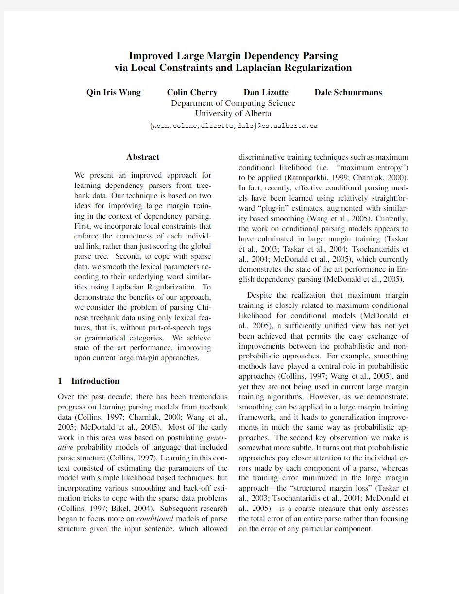
Figure1:A dependency tree
In this paper,we make two contributions to the large margin approach to learning parsers from su-pervised data.First,we show that smoothing based on lexical similarity is not only possible in the large margin framework,but more importantly,allows better generalization to new words not encountered during training.Second,we show that the large mar-gin training objective can be signi?cantly re?ned to assess the error of each component of a given parse, rather than just assess a global score.We show that these two extensions together lead to greater train-ing accuracy and better generalization to novel input sentences than current large margin methods.
To demonstrate the bene?t of combining useful learning principles from both the probabilistic and large margin frameworks,we consider the prob-lem of learning a dependency parser for Chinese. This is an interesting test domain because Chinese does not have clearly de?ned parts-of-speech,which makes lexical smoothing one of the most natural ap-proaches to achieving reasonable results(Wang et al.,2005).
2Lexicalized Dependency Parsing
A dependency tree speci?es which words in a sen-tence are directly related.That is,the dependency structure of a sentence is a directed tree where the nodes are the words in the sentence and links rep-resent the direct dependency relationships between the words;see Figure1.There has been a grow-ing interest in dependency parsing in recent years. (Fox,2002)found that the dependency structures of a pair of translated sentences have a greater de-gree of cohesion than phrase structures.(Cherry and Lin,2003)exploited such cohesion between the de-pendency structures to improve the quality of word alignment of parallel sentences.Dependency rela-tions have also been found to be useful in informa-tion extraction(Culotta and Sorensen,2004;Yan-garber et al.,2000).
A key aspect of a dependency tree is that it does not necessarily report parts-of-speech or phrase la-bels.Not requiring parts-of-speech is especially bene?cial for languages such as Chinese,where parts-of-speech are not as clearly de?ned as En-glish.In Chinese,clear indicators of a word’s part-of-speech such as suf?xes“-ment”,“-ous”or func-tion words such as“the”,are largely absent.One of our motivating goals is to develop an approach to learning dependency parsers that is strictly lexical. Hence the parser can be trained with a treebank that only contains the dependency relationships,making annotation much easier.
Of course,training a parser with bare word-to-word relationships presents a serious challenge due to data sparseness.It was found in(Bikel,2004)that Collins’parser made use of bi-lexical statistics only 1.49%of the time.The parser has to compute back-off probability using parts-of-speech in vast majority of the cases.In fact,it was found in(Gildea,2001) that the removal of bi-lexical statistics from a state of the art PCFG parser resulted in very little change in the output.(Klein and Manning,2003)presented an unlexicalized parser that eliminated all lexical-ized parameters.Its performance was close to the state of the art lexicalized parsers. Nevertheless,in this paper we follow the re-cent work of(Wang et al.,2005)and consider a completely lexicalized parser that uses no parts-of-speech or grammatical categories of any kind.Even though a part-of-speech lexicon has always been considered to be necessary in any natural language parser,(Wang et al.,2005)showed that distributional word similarities from a large unannotated corpus can be used to supplant part-of-speech smoothing with word similarity smoothing,to still achieve state of the art dependency parsing accuracy for Chinese. Before discussing our modi?cations to large mar-gin training for parsing in detail,we?rst present the dependency parsing model we use.We then give a brief overview of large margin training,and then present our two modi?cations.Subsequently,we present our experimental results on fully lexical de-pendency parsing for Chinese.
3Dependency Parsing Model
Given a sentence W=(w1,...,w n)we are in-terested in computing a directed dependency tree,
T,over W.In particular,we assume that a di-rected dependency tree T consists of ordered pairs (w i→w j)of words in W such that each word ap-pears in at least one pair and each word has in-degree at most one.Dependency trees are usually assumed to be projective(no crossing arcs),which means that if there is an arc(w i→w j),then w i is an ancestor of all the words between w i and w j.LetΦ(W)de-note the set of all the directed,projective trees that span W.
Given an input sentence W,we would like to be able to compute the best parse;that is,a projective tree,T∈Φ(W),that obtains the highest“score”. In particular,we follow(Eisner,1996;Eisner and Satta,1999;McDonald et al.,2005)and assume that the score of a complete spanning tree T for a given sentence,whether probabilistically motivated or not, can be decomposed as a sum of local scores for each link(a word pair).In which case,the parsing prob-lem reduces to
T?=arg max
T∈Φ(W)
(w i→w j)∈T
s(w i→w j)(1)
where the score s(w i→w j)can depend on any measurable property of w i and w j within the tree T.This formulation is suf?ciently general to capture most dependency parsing models,including proba-bilistic dependency models(Wang et al.,2005;Eis-ner,1996)as well as non-probabilistic models(Mc-Donald et al.,2005).For standard scoring functions, parsing requires an O(n3)dynamic programming algorithm to compute a projective tree that obtains the maximum score(Eisner and Satta,1999;Wang et al.,2005;McDonald et al.,2005).
For the purpose of learning,we decompose each link score into a weighted linear combination of fea-tures
s(w i→w j)=θ f(w i→w j)(2) whereθare the weight parameters to be estimated during training.
Of course,the speci?c features used in any real situation are critical for obtaining a reasonable de-pendency parser.The natural sets of features to con-sider in this setting are very large,consisting at the very least of features indexed by all possible lexical items(words).For example,natural features to use for dependency parsing are indicators of each possi-ble word pair
f uv(w i→w j)=1(w
i=u)
1(w
j=v) which allows one to represent the tendency of two words,u and v,to be directly linked in a parse.In this case,there is a corresponding parameterθuv to be learned for each word pair,which represents the strength of the possible linkage.
A large number of features leads to a serious risk of over-?tting due to sparse data problems.The stan-dard mechanisms for mitigating such effects are to combine features via abstraction(https://www.doczj.com/doc/e33182179.html,ing parts-of-speech)or smoothing(https://www.doczj.com/doc/e33182179.html,ing word similarity based smoothing).For abstraction,a common strat-egy is to use parts-of-speech to compress the feature set,for example by only considering the tag of the parent
f pv(w i→w j)=1(pos(w
i)=p)
1(w
j=v) However,rather than use abstraction,we will follow a purely lexical approach and only consider features that are directly computable from the words them-selves(or statistical quantities that are directly mea-surable from these words).
In general,the most important aspect of a link feature is simply that it measures something about a candidate word pair that is predictive of whether the words will actually be linked in a given sen-tence.Thus,many other natural features,beyond parts-of-speech and abstract grammatical categories, immediately suggest themselves as being predictive of link existence.For example,one very useful fea-ture is simply the degree of association between the two words as measured by their pointwise mutual information
f PMI(w i→w j)=PMI(w i,w j) (We describe in Section6below how we compute this association measure on an auxiliary corpus of unannotated text.)Another useful link feature is simply the distance between the two words in the sentence;that is,how many words they have be-tween them
f dist(w i→w j)=|position(w i)?position(w j)|
In fact,the likelihood of a direct link between two words diminishes quickly with distance,which mo-tivates using more rapidly increasing functions of distance,such as the square
f dist2(w i→w j)=(position(w i)?position(w j))2 In our experiments below,we used only these sim-ple,lexically determined features,{f uv},f PMI,f dist and f dist2,without the parts-of-speech{f pv}.Cur-rently,we only use undirected forms of these fea-tures,where,for example,f uv=f vu for all pairs (or,put another way,we tie the parametersθuv=θvu together for all u,v).Ideally,we would like to use directed features,but we have already found that these simple undirected features permit state of the art accuracy in predicting(undirected)depen-dencies.Nevertheless,extendin
g our approac
h to di-rected features and contextual features,as in(Wang et al.,2005),remains an important direction for fu-ture research.
4Large Margin Training
Given a training set of sentences annotated with their correct dependency parses,(W1,T1),...,(W N,T N), the goal of learning is to estimate the parameters of the parsing model,θ.In particular,we seek values for the parameters that can accurately reconstruct the training parses,but more importantly,are also able to accurately predict the dependency parse structure on future test sentences.
To trainθwe follow the large margin training ap-proach of(Taskar et al.,2003;Tsochantaridis et al., 2004),which has been applied with great success to dependency parsing(Taskar et al.,2004;McDonald et al.,2005).Large margin training can be expressed as minimizing a regularized loss(Hastie et al.,2004)
min θβ
2
θ θ+e ξsubject to(4)
ξi≥?(T i,L i)+s(θ,L i)?s(θ,T i)
for all i,L i∈Φ(W i)
which corresponds to the training problem posed in
(McDonald et al.,2005).
Unfortunately,the quadratic program(4)has three
problems one must address.First,there are expo-
nentially many constraints—corresponding to each
possible parse of each training sentence—which
forces one to use alternative training procedures,
such as incremental constraint generation,to slowly
converge to a solution(McDonald et al.,2005;
Tsochantaridis et al.,2004).Second,and related,
the original loss(4)is only evaluated at the global
parse tree level,and is not targeted at penalizing any
speci?c component in an incorrect parse.Although
(McDonald et al.,2005)explicitly describes this
as an advantage over previous approaches(Ratna-
parkhi,1999;Yamada and Matsumoto,2003),below
we?nd that changing the loss to enforce a more de-
tailed set of constraints leads to a more effective ap-
proach.Third,given the large number of bi-lexical
features{f uv}in our model,solving(4)directly will
over-?t any reasonable training corpus.(Moreover,
using a largeβto shrink theθvalues does not mit-
igate the sparse data problem introduced by having
so many features.)We now present our re?nements
that address each of these issues in turn.
5Training with Local Constraints
We are initially focusing on training on just an
undirected link model,where each parameter in the
model is a weightθww between two words,w and
w ,respectively.Since links are undirected,these
weights are symmetricθww =θw w,and we can
also write the score in an undirected fashion as:
s(w,w )=θ f(w,w ).The main advantage of
working with the undirected link model is that the
constraints needed to ensure correct parses on the
training data are much easier to specify in this case.
Ignoring the projective(no crossing arcs)constraint
for the moment,an undirected dependency parse can
be equated with a maximum score spanning tree of a sentence.Given a target parse,the set of constraints needed to ensure the target parse is in fact the max-imum score spanning tree under the weightsθ,by at least a minimum amount,is a simple set of lin-ear constraints:for any edge w1w2that is not in the target parse,one simply adds two constraints
θ f(w1,w 1)≥θ f(w1,w2)+1
θ f(w2,w 2)≥θ f(w1,w2)+1(5)
where the edges w1w
1and w2w
2
are the adjacent
edges that actually occur in the target parse that are also on the path between w1and w2.(These would have to be the only such edges,or there would be a loop in the parse tree.)These constraints behave very naturally by forcing the weight of an omitted edge to be smaller than the adjacent included edges that would form a loop,which ensures that the omit-ted edge would not be added to the maximum score spanning tree before the included edges.
In this way,one can simply accumulate the set of linear constraints(5)for every edge that fails to be included in the target parse for the sentences where it is a candidate.We denote this set of constraints by A={θ f(w1,w 1)≥θ f(w1,w2)+1} Importantly,the constraint set A is convex in the link weight parametersθ,as it consists only of linear constraints.
Ignoring the non-crossing condition,the con-straint set A is exact.However,because of the non-crossing condition,the constraint set A is more restrictive than necessary.For example,consider the word sequence...w i w i+1w i+2w i+3...,where the edge w i+1w i+3is in the target parse.Then the edge w i w i+2can be ruled out of the parse in one of two ways:it can be ruled out by making its score less than the adjacent scores as speci?ed in(5),or it can be ruled out by making its score smaller than the score of w i+1w i+3.Thus,the exact constraint contains a disjunction of two different constraints, which creates a non-convex constraint inθ.(The union of two convex sets is not necessarily convex.) This is a weakening of the original constraint set A. Unfortunately,this means that,given a large train-ing corpus,the constraint set A can easily become infeasible.
Nevertheless,the constraints in A capture much of the relevant structure in the data,and are easy to enforce.Therefore,we wish to maintain them. However,rather than impose the constraints exactly, we enforce them approximately through the intro-duction of slack variablesξ.The relaxed constraints can then be expressed as
θ f(w1,w 1)≥θ f(w1,w2)+1?ξw
1w2,w1w 1
(6) and therefore a maximum soft margin solution can then be expressed as a quadratic program
min
θ,ξ
β
The basic intuition behind similarity smoothing is that words that tend to appear in the same con-texts tend to have similar meanings.This is known as the Distributional Hypothesis in linguistics(Har-ris,1968).For example,the words test and exam are similar because both of them can follow verbs such as administer,cancel,cheat on,conduct,etc. Many methods have been proposed to compute distributional similarity between words,e.g.,(Hin-dle,1990;Pereira et al.,1993;Grefenstette,1994;
Lin,1998).Almost all of the methods represent a word by a feature vector where each feature corre-sponds to a type of context in which the word ap-peared.They differ in how the feature vectors are constructed and how the similarity between two fea-ture vectors is computed.
In our approach below,we de?ne the features of a word w to be the set of words that occurred within a small window of w in a large corpus.The con-text window of w consists of the closest non-stop-word on each side of w and the stop-words in be-tween.The value of a feature w is de?ned as the pointwise mutual information between the w and w:PMI(w ,w)=log(P(w,w )
S(w1,w2)S(w 1,w 2)(8) where S(w1,w2)is de?ned as in Section6above. Then,instead of just solving the constraint system (7)we can also ensure that similar links take on sim-ilar parameter values by introducing a penalty on their deviations that is weighted by their similarity value.Speci?cally,we use
w1w
1
w2w
2
S(w1w 1,w2w 2)(θw
1w 1
?θw
2w 2
)2
=2θ L(S)θ (9) Here L(S)is the Laplacian matrix of S,which is de?ned by L(S)=D(S)?S where D(S) is a diagonal matrix such that D w
1w 1,w1w 1
= w2w 2S(w1w 1,w2w 2).Also,θ corresponds to the
vector of bi-lexical parameters.In this penalty func-tion,if two edges w1w
1
and w2w
2
have a high sim-ilarity value,their parameters will be encouraged to take on similar values.By contrast,if two edges have low similarity,then there will be little mutual attraction on their parameter values.
Note,however,that we do not smooth the param-eters,θPMI,θdist,θdist2,corresponding to the point-wise mutual information,distance,and squared dis-tance features described in Section5,respectively. We only apply similarity smoothing to the bi-lexical parameters.
The Laplacian regularizer(9)provides a natural smoother for the bi-lexical parameter estimates that takes into account valuable word similarity informa-tion computed as above.The Laplacian regularizer also has a signi?cant computational advantage:it is guaranteed to be a convex quadratic function of the parameters(Zhu et al.,2003).Therefore,by com-bining the constraint system(7)with the Laplacian smoother(9),we can obtain a convex optimization
Table1:Accuracy Results on CTB Test Set
Features used Trained w/
global loss Pairs0.6426
+Lap0.6506
+Dist0.6546
+Lap+Dist0.6586
+MI+Dist0.6707
+Lap+MI+Dist0.6827
Trained w/
local loss
0.5688
0.4935
0.6130
0.5299
0.6182
0.5662 procedure for estimating the link parameters
min θ,ξβ
Trained w/
local loss
0.8393
0.7216
0.8376
0.7216
0.7985
0.7062
in CTB are constituency structures.We converted
them into dependency trees using the same method
and head-?nding rules as in(Bikel,2004).Follow-
ing(Bikel,2004),we used Sections1-270for train-
ing,Sections271-300for testing and Sections301-
325for development.We experimented with two
sets of data:CTB-10and CTB-15,which contains
sentences with no more than10and15words re-
spectively.Table1,Table2and Table3show our
experimental results trained and evaluated on Chi-
nese Treebank sentences of length no more than10,
using the standard split.For any unseen link in the
new sentences,the weight is computed as the simi-
larity weighted average of similar links seen in the
training corpus.The regularization parameterβwas
set by5-fold cross-validation on the training set.
We evaluate parsing accuracy by comparing the
undirected dependency links in the parser outputs
against the undirected links in the treebank.We de-
?ne the accuracy of the parser to be the percentage
of correct dependency links among the total set of
dependency links created by the parser.
Table1and Table2show that training based on
the more re?ned local loss is far superior to training
with the global loss of standard large margin train-
ing,on both the test and development sets.Parsing
accuracy also appears to increase with the introduc-
tion of each new feature.Notably,the pointwise mu-
tual information and distance features signi?cantly
improve parsing accuracy—and yet we know of no
other research that has investigated these features in
this context.Finally,we note that Laplacian regular-
ization improved performance as expected,but not
for the global loss,where it appears to systemati-
cally degrade performance(n/a results did not com-
plete in time).It seems that the global loss model
may have been over-regularized(Table3).However,
we have picked theβparameter which gave us the
best results in our experiments.One possible ex-planation for this phenomenon is that the interaction between the Laplacian regularization in training and the similarity smoothing in parsing,since distribu-tional word similarities are used in both cases. Finally,we compared our results to the probabilis-tic parsing approach of(Wang et al.,2005),which on this data obtained accuracies of0.7631on the CTB test set and0.6104on the development set.How-ever,we are using a much simpler feature set here. 9Conclusion
We have presented two improvements to the stan-dard large margin training approach for dependency parsing.To cope with the sparse data problem,we smooth the parameters according to their underlying word similarities by introducing a Laplacian regular-izer.More signi?cantly,we use more re?ned local constraints in the large margin criterion,rather than the global parse-level losses that are commonly con-sidered.We achieve state of the art parsing accuracy for predicting undirected dependencies in test data, competitive with previous large margin and previous probabilistic approaches in our experiments. Much work remains to be done.One extension is to consider directed features,and contextual fea-tures like those used in current probabilistic parsers (Wang et al.,2005).We would also like to apply our approach to parsing English,investigate the confu-sion shown in Table3more carefully,and possibly re-investigate the use of parts-of-speech features in this context.
References
Dan Bikel.2004.Intricacies of collins’parsing https://www.doczj.com/doc/e33182179.html,-putational Linguistics,30(4).
Eugene Charniak.2000.A maximum entropy inspired parser. In Proceedings of NAACL-2000,pages132–139.
Colin Cherry and Dekang Lin.2003.A probability model to improve word alignment.In Proceedings of ACL-2003. M.J.Collins.1997.Three generative,lexicalized models for statistical parsing.In Proceedings of ACL-1997.
Aron Culotta and Jeffery Sorensen.2004.Dependency tree kernels for relation extraction.In Proceedings of ACL-2004. J.Eisner and G.Satta.1999.Ef?cient parsing for bilexical context-free grammars and head-automaton grammars.In Proceedings of ACL-1999.J.Eisner.1996.Three new probabilistic models for depen-dency parsing:An exploration.In Proc.of COLING-1996. Heidi J.Fox.2002.Phrasal cohesion and statistical machine translation.In Proceedings of EMNLP-2002.
Daniel Gildea.2001.Corpus variation and parser performance. In Proceedings of EMNLP-2001,Pittsburgh,PA. Gregory Grefenstette.1994.Explorations in Automatic The-saurus Discovery.Kluwer Academic Press,Boston,MA. Zelig S.Harris.1968.Mathematical Structures of Language. Wiley,New York.
T.Hastie,S.Rosset,R.Tibshirani,and J.Zhu.2004.The entire regularization path for the support vector machine.JMLR,5. Donald Hindle.1990.Noun classi?cation from predicate-argument structures.In Proceedings of ACL-1990.
Dan Klein and Christopher D.Manning.2003.Accurate un-lexicalized parsing.In Proceedings of ACL-2003. Dekang Lin.1998.Automatic retrieval and clustering of simi-lar words.In Proceedings of COLING/ACL-1998.
R.McDonald,K.Crammer,and F.Pereira.2005.Online large-margin training of dependency parsers.In Proceedings of ACL-2005.
F.Pereira,N.Tishby,and L.Lee.1993.Distributional cluster-ing of english words.In Proceedings of ACL-1993. Adwait Ratnaparkhi.1999.Learning to parse natural language with maximum entropy models.Machine Learning,34(1-3).
B.Taskar,
C.Guestrin,and
D.Koller.2003.Max-margin markov networks.In Proc.of NIPS-2003.
B.Taskar,D.Klein,M.Collins,D.Koller,and
C.Manning. 2004.Max-margin parsing.In Proceedings of EMNLP. I.Tsochantaridis,T.Hofmann,T.Joachims,and Y.Altun. 2004.Support vector machine learning for interdependent and structured output spaces.In Proceedings of ICML-2004. Q.Wang,
D.Schuurmans,and D.Lin.2005.Strictly lexical dependency parsing.In Proceedings of IWPT-2005.
N.Xue,F.Xia,F.Chiou,and M.Palmer.2004.The penn chi-nese treebank:Phrase structure annotation of a large corpus. Natural Language Engineering,10(4):1–30.
H.Yamada and Y.Matsumoto.2003.Statistical dependency analysis with support vector machines.In Proceedings of IWPT-2003.
R.Yangarber,R.Grishman,P.Tapanainen,and S.Huttunen. 2000.Unsupervised discovery of scenario-level patterns for information extraction.In Proceedings of ANLP/NAACL-2000.
Xiaojin Zhu,John Lafferty,and Zoublin Ghahramani.2003. Semi-supervised learning using gaussian?elds and harmonic functions.In Proceedings of ICML-2003.
Matlab 第十章作业 10.4考虑一个单位负反馈控制系统,其前向通道传递函数为: )5s (s 1)s (G 20+= 试应用Bode 图法设计一个超前校正装置)1 1()(++=Ts Ts K s G c c αα 使得校正后系统的相角裕度 50=γ,幅值裕度dB 10K g ≥,带宽 s /rad 2~1b =ω。其中,10<<α。试问已校正系统的谐振峰值r M 和谐振角频率 r ω的值各为多少? 解: ① 先建立超前校正函数fg_lead_pm (wc 未知) 函数语句如下 function [ngc,dgc]=fg_lead_pm(ng0,dg0,Pm,w) [mu,pu]=bode(ng0,dg0,w); [gm,pm,wcg,wcp]=margin(mu,pu,w); alf=ceil(Pm-pm+5); phi=(alf)*pi/180; a=(1+sin(phi))/(1-sin(phi)) ; a1=1/a%求参数α dbmu=20*log10(mu); mm=-10*log10(a); wgc=spline(dbmu,w,mm); T=1/(wgc*sqrt(a)); ngc=[a*T,1]; dgc=[T,1]; ② 建立M 文件l104其语句如下 ng0=[1];dg0=conv([1,0],conv([1,0],[1,5])); t=[0:0.01:5]; w=logspace(-3,2); g0=tf(ng0,dg0) b1=feedback(g0,1)%校正前系统闭环传函 [gm,pm,wcg,wcp]=margin(g0)%校正前参数 Pm=50; [ng1,dg1]=fg_lead_pm(ng0,dg0,Pm,w);%利用超前校正进行校正 g1=tf(ng1,dg1);%校正环节传递函数 g2=g0*g1;%校正后前向通道传函 [gm1,pm1,wcg1,wcp1]=margin(g2)%校正后系统参数 km1=20*log(gm1)%校正后系统幅值裕度工程表示 b2=feedback(g2,1);%校正后系统闭环传函
交易开拓者函数一览表(文华对照) 交易开拓者文华 数学函数 绝对值Abs ABS(X) 反余弦值Acos ACOS(X) 反双曲余弦值Acosh 反正弦值Asin ASIN(X) 反双曲正弦值Asinh 反正切值Atan ATAN(X) 给定的X及Y坐标值的反正切值Atan2 反双曲正切值Atanh 沿绝对值增大方向按基数舍入Ceiling 从给定数目的对象集合中提取若 Combin 干对象的组合数 余弦值Cos COS(X) 双曲余弦值Cosh 余切值Ctan 沿绝对值增大方向取整后最接近 Even 的偶数 e的N次幂Exp EXP(X) 数的阶乘Fact 沿绝对值减少的方向去尾舍入Floor
实数舍入后的小数值FracPart 实数舍入后的整数值IntPart 自然对数Ln LN(X) 对数Log LOG(X) 余数Mod MOD(A,B) 负绝对值Neq 指定数值舍入后的奇数Odd 返回PI Pi 给定数字的乘幂Power POW(A,B) 随机数Rand 按指定位数舍入Round 靠近零值,舍入数字RoundDown 远离零值,舍入数字RoundUp 数字的符号Sign SGN(X) 正弦值Sin 双曲正弦值Sinh SIN(X) 平方Sqr SQUARE(X) 正平方根Sqrt SQRT(X) 正切值Tan TAN(X) 双曲正切值Tanh 取整Trunc INTPART(X) 字符串函数
测试是否相同Exact 返回字符串中的字符数Len 大写转小写Lower 数字转化为字符串Text 取出文本两边的空格Trim 小写转大写Upper 文字转化为数字Value 颜色函数 黑色Black COLORBLACK 蓝色Blue COLORBLUE 青色Cyan COLORCYAN 茶色DarkBrown 深青色DarkCyan 深灰色DarkGray 深绿色DarkGreen 深褐色DarkMagenta 深红色DarkRed 默认颜色DefaultColor 绿色Green COLORGREEN 浅灰色LightGray COLORLIGHTGREY 紫红色Magenta COLORMAGENTA 红色Red COLORRED
halcon算子中文解释 comment ( : : Comment : ) 注释语句 exit ( : : : ) 退出函数 open_file ( : : FileName, FileType : FileHandle ) 创建('output' or 'append' )或者打开(output )文本文件 fwrite_string ( : : FileHandle, String : ) 写入string dev_close_window ( : : : ) 关闭活跃的图形窗口。 read_image ( : Image : FileName : ) ;加载图片 get_image_pointer1 ( Image : : : Pointer, Type, Width, Height ) 获得图像的数据。如:类型(= ' 字节',' ' ',uint2 int2 等等) 和图像的尺寸( 的宽度和高度) dev_open_window( : :Row,Column,WidthHeight,Background :WindowHandle ) 打开一个图形的窗口。 dev_set_part ( : : Row1, Column1, Row2, Column2 : ) 修改图像显示的位置 dev_set_draw (’fill’)填满选择的区域 dev_set_draw (’margin’)显示的对象只有边缘线, dev_set_line_width (3) 线宽用Line Width 指定 threshold ( Image : Region : MinGray, MaxGray : ) 选取从输入图像灰度值的g 满足下列条件:MinGray < = g < = MaxGray 的像素。 dev_set_colored (number) 显示region 是用到的颜色数目 dev_set_color ( : : ColorName : ) 指定颜色 connection ( Region : ConnectedRegions : : ) 合并所有选定像素触摸相互连通区 fill_up ( Region : RegionFillUp : : ) 填补选择区域中空洞的部分 fill_up_shape ( Region : RegionFillUp : Feature, Min, Max : ) select_shape ( Regions : SelectedRegions : Features, Operation, Min, Max : ) 选择带有某些特征的区域,Operation 是运算,如“与”“或” smallest_rectangle1 ( Regions : : : Row1, Column1, Row2, Column2 ) 以矩形像素坐标的角落,Column1,Row2(Row1,Column2) 计算矩形区域( 平行输入坐标轴) 。 dev_display ( Object : : : ) 显示图片 disp_rectangle1 ( : : WindowHandle, Row1, Column1, Row2, Column2 : ) 显示的矩形排列成的。disp_rectangle1 显示一个或多个矩形窗口的产量。描述一个矩形左上角(Row1,Column1) 和右下角(Row2,Column2) 。显示效果如图1. texture_laws ( Image : ImageT exture : FilterTypes, Shift, FilterSize : ) texture_laws 实行纹理变换图像FilterTypes: 预置的过滤器Shift :减少灰度变化FilterSize :过滤的尺寸 mean_image ( Image : ImageMean : MaskWidth, MaskHeight : ) 平滑图像, 原始灰度值的平均数MaskWidth: 过滤器的宽度面具 bin_threshold ( Image : Region : : ) 自动确定阈值 Region: 黑暗的区域的图像 dyn_threshold ( OrigImage, ThresholdImage : RegionDynThresh : Offset, LightDark : ) 比较两个像素的图像像素RegionDynThresh(Out) 分割区域Offset: 减少噪音引起的问题LightDark 提取光明、黑暗或类似的地方? dilation_circle ( Region : RegionDilation : Radius : ) 扩张有一个圆形结构元素的地区Radius 圆半径 complement ( Region : RegionComplement : : ) 返还补充的区域 reduce_domain ( Image, Region : ImageReduced : : ) 减少定义领域的图像
扬州大学实验报告纸 实验名称:7.2 控制原理仿真实验 班级:建电1102 姓名:葛嘉新 学号:111705205 7.2.4 控制系统的博德图 1.实验目的 (1)利用计算机作出开环系统的博德图; (2)观察记录控制系统的开环频域性能; (3)控制系统的开环频率特性分析。 2.实验步骤 (1)运行MATLAB (2)练习相关m 函数 1)博德图绘图函数 bode(sys) bode(sys,{wmin,wmax}) bode(sys,w) [m,p,w]=bode(sys) 函数功能:对数频率特性作图函数,即博德图作图。 2)对数分度函数 logspace(d1,d2) logspace(d1,d2,n) 函数功能:产生对数分度向量。 3)稳定裕度函数 margin(sys) [Gm,Pm,wg,wp]=margin(sys) [Gm,Pm,wg,wp]=margin(m,p,w) 函数功能:计算系统的稳定裕度、相位裕度Gm 和幅值裕度Pm 。 3.实验内容 (1)221 (s), 21 G T S TS ζ= ++{0.1 2,1,0.5,0.1,0.01T ζ== (分别作图并保持) >> n=1; >> d1=[0.01 0.4 1];d2=[0.01 0.2 1];d3=[0.01 0.1 1]; >> d4=[0.01 0.02 1];d5=[0.01 0.002 1]; %建立系统模型 >> bode(n,d1);hold on; %作博德图,并保持作图 >> bode(n,d2);bode(n,d3);bode(n,d4);bode(n,d5) >> grid %各系统博德图和网格线,如图1 -80-60-40-2002040M a g n i t u d e (d B ) 10 -1 10 10 1 10 2 10 3 -180-135-90-45 0P h a s e (d e g ) Bode Diagram Frequency (rad/sec) 图1 图1说明: 幅频特性中,ω=10时,最小的是ζ=2,最大的是ζ=0.01。相频特性中,ω=10时,越变最小的是ζ=2,越变最大的是ζ=0.01。 (2) 31.6 (s)(0.01+1)(0.1s+1) G s s = 要求: 1)作博德图,在曲线上标出: 幅频特性——初始段斜率、高频段斜率、开环截止频率、中频段穿越斜率。 相频特性——低频段渐进相位角、高频段渐进相位角、-180°线的穿越频率。 2)由稳定裕度命令计算系统的稳定裕度Lg 和γc ,并确定系统的稳定性; 3)在图上作近似折线特性相比较。 >> n=31.6;d=conv([0.01 1 0],[0.1 1]); >> sys=tf(n,d); >> margin(sys) >> hold on >> grid %博德图如下页图2
实验一、MATLAB 语言的符号运算 1、实验目的 (1)学习MATLAB 语言的基本符号运算; (2)学习MATLAB 语言的矩阵符号运算; 2、实验内容 (1)基本符号运算 1) 符号微分、积分 syms t f1=sin (2*t); df1=diff(f1) if1=int (f1) 2) 泰勒级数展开 tf1=taylor (f1,8) 3) 符号代数方程求解 syms a b c x; f=a*x^2+b*x+c; ef=solve (f) 4) 符号微分方程求解 f=’D2x+2*Dx+10*x=0’;g=’Dx(0)=1,x(0)=0’; dfg=dsolve(f,g) 求满足初始条件的二阶常系数齐次微分方程的特解: 2|,4|,020'022-===++==t t s s s dt ds dt s d 5) 积分变换 syms t f1=exp(-2*t)*sin (5*t)
F1=laplace(f1) F2=ilaplace(F1) (2) 符号矩阵运算 1)创建与修改符号矩阵 G1=sym(‘[1/(s+1),s/(s+1)/(s+2);1/(s+1)/(s+2),s/(s+2)]’) G2=subs(G1,G1(2,2),’0’) G3=G1(1,1) 2)常规符号运算 syms s d1=1/(s+1);d2=1/(s+2);d=d1*d2 ad=sym(‘[s+1 s;0 s+2]’); G=d*ad n1=[1 2 3 4 5];n2=[1 2 3]; p1=poly2sym (n1);p2=poly2sym(n2); p=p1+p2 pn=sym2poly(p) 实验二、控制系统的阶跃响应 一、实验目的 (1)观察学习控制系统的单位阶跃响应; (2)记录单位阶跃响应曲线 (3)观察时间响应分析的一般方法 二、实验步骤 (1)运行MATLAB
1. 成绩: 报告50%:最多三页,不许打印。注意格式填写全,否则扣分;主体部分包括: 实验目的,实验内容,源程序及必要的注释,实验总结) 实验50%:(1)纪律10%, ⑵回答问题10%:①必答题,抽到必答。主要考察考察预习情况和对 相应理论掌握情况 ②选答题,答对加分,答错不扣分。与课堂内容有 关,略有深度,依学号末位随机抽取。每次人数不 定。 ⑶实验能力30%:能独立完成实验,且完成用时较少者分最高。 2. 交报告时间:二次上课时交第一次报告,依此类推,最后一次由班长收齐交到 我办公室教6-816 研究自控课程的意义:苏27,901雷达,孵化器 实验一 系统的动态响应 一、实验目的 1、掌握一阶系统和二阶系统的非周期信号响应。 2、理解二阶系统的无阻尼、欠阻尼、临界阻尼和过阻尼。 3、掌握分析系统稳定性、瞬态过程和稳态误差的方法。 4、理解高阶系统的主导极点对系统特性的影响。 5、理解系统的零点对系统动态特性的影响。 二、实验内容(讲一个(M 文件和SIMULINK 两种方法),练一个,报告上写一个) 1、(讲解演示) 系统框图如下所示, (1) 若2()210 G s s s =++,求系统的单位阶跃响应。 (2)分析系统的稳定性。(举例说明研究稳定性的意义,判断准则) 我们采用matlab 进行分析步骤 (1)采用M 文件求解
步骤:a.新建一个m文件 b.输入系统的传递函数 c.分析系统的稳定性(根据线性系统稳定的充分必要条件:闭环系统特征方程D(s)=0的所有根均具有负实部,只要求出系统极点,由其实部可得到系统稳定性) d.输入为单位阶跃信号时,求系统的响应 example1.m: numg=[10] %分子多项式 deng=[1 2 10] %分母多项式 sys1=tf(numg,deng) %tf函数构造开环传递函数G(s) sys=feedback(sys1,1) % 求得闭环传递函数 pole(sys) % 求系统极点,即特征方程的根 step(sys) % 求阶跃响应 grid on 运行结果:ans = 极点 -1.0000 + 4.3589i -1.0000 - 4.3589i
词汇 第一章 自动控制 ( Automatic Control) :是指在没有人直接参与的条件下,利用控制装置使被控对象的某些物理量(或状态)自动地按照预定的规律去运行。 开环控制 ( open loop control ):开环控制是最简单的一种控制方式。它的特点是,按照控制信息传递的路径,控制量与被控制量之间只有前向通路而没有反馈通路。也就是说,控制作用的传递路径不是闭合的,故称为开环。 闭环控制 ( closed loop control) :凡是将系统的输出量反送至输入端,对系统的控制作用产生直接的影响,都称为闭环控制系统或反馈控制 Feedback Control 系统。这种自成循环的控制作用,使信息的传递路径形成了一个闭合的环路,故称为闭环。 复合控制 ( compound control ):是开、闭环控制相结合的一种控制方式。 被控对象:指需要给以控制的机器、设备或生产过程。被控对象是控制系统的主体,例如火箭、锅炉、机器人、电冰箱等。控制装置则指对被控对象起控制作用的设备总体,有测量变换部件、放大部件和执行装置。 被控量 (controlled variable ) :指被控对象中要求保持给定值、要按给定规律变化的物理量。被控量又称输出量、输出信号。 给定值 (set value ) :是作用于自动控制系统的输入端并作为控制依据的物理量。给定值又称输入信号、输入指令、参考输入。 干扰 (disturbance) :除给定值之外,凡能引起被控量变化的因素,都是干扰。干扰又称扰动。 第二章 数学模型 (mathematical model) :是描述系统内部物理量(或变量)之间动态关系的数学表达式。 传递函数 ( transfer function) :线性定常系统在零初始条件下,输出量的拉氏变换与输入量的拉氏变换之比,称为传递函数。 零点极点 (z ero and pole) :分子多项式的零点(分子多项式的根)称为传递函数的零点;分母多项式的零点(分母多项式的根)称为传递函数的极点。 状态空间表达式 (state space model) :由状态方程与输出方程组成,状态方程是各状态变量的一阶导数与状态、输入之间的一阶微分方程组。输出方程是系统输出与状态、输入之间的关系方程。 结构图 (block diagram) :将传递函数与第一章介绍的定性描述系统的方框图结合起来,就产生了一种描述系统动态性能及数学结构的方框图,称之为系统的动态结构图。 信号流图 (signal flow diagram) :是表示复杂控制系统中变量间相互关系的另一种图解法,由节点和支路组成。 梅逊公式 (Mason's gain formula) :利用梅逊增益公式,可以直接得到系统输出量与输入变量之间的传递函数。 第三章 时域 (time domain) :一种数学域,与频域相区别,用时间 t 和时间响应来描述系统。 一阶系统 ( first order system) :控制系统的运动方程为一阶微分方程,称为一阶系统。 二阶系统 ( s econd order system) :控制系统的运动方程为二阶微分方程,称为二阶系统。 单位阶跃响应 ( unit step response) :系统在零状态条件下,在单位阶跃信号作用下的响应称单位阶跃响应。 阻尼比ζ (damping ratio) :与二阶系统的特征根在 S 平面上的位置密切相关,不同阻尼比
? 在下一行显示表达式串 ?? 在当前行显示表达式串 @... 将数据按用户设定的格式显示在屏幕上或在打印机上打印 ACCEPT 把一个字符串赋给内存变量 APPEND 给数据库文件追加记录 APPEND FROM 从其它库文件将记录添加到数据库文件中 AVERAGE 计算数值表达式的算术平均值 BROWSE 全屏幕显示和编辑数据库记录 CALL 运行内存中的二进制文件 CANCEL 终止程序执行,返回圆点提示符 CASE 在多重选择语句中,指定一个条件 CHANGE 对数据库中的指定字段和记录进行编辑 CLEAR 清洁屏幕,将光标移动到屏幕左上角 CLEAR ALL 关闭所有打开的文件,释放所有内存变量,选择1号工作区 CLEAR FIELDS 清除用SET FIELDS TO命令建立的字段名表 CLEAR GETS 从全屏幕READ中释放任何当前GET语句的变量CLEAR MEMORY 清除当前所有内存变量 CLEAR PROGRAM 清除程序缓冲区 CLEAR TYPEAHEAD 清除键盘缓冲区 CLOSE 关闭指定类型文件 CONTINUE 把记录指针指到下一个满足LOCATE命令给定条件
的记录,在LOCATE命令后出现。无LOCATE则出错 COPY TO 将使用的数据库文件复制另一个库文件或文本文件 COPY FILE 复制任何类型的文件 COPY STRUCTURE EXTENED TO 当前库文件的结构作为记录,建立一个新的库文件 COPY STRUCTURE TO 将正在使用的库文件的结构复制到目的库文件中 COUNT 计算给定范围内指定记录的个数 CREATE 定义一个新数据库文件结构并将其登记到目录中 CREATE FROM 根据库结构文件建立一个新的库文件 CREATE LABEL 建立并编辑一个标签格式文件 CREATE REPORT 建立宾编辑一个报表格式文件 DELETE 给指定的记录加上删除标记 DELETE FILE 删除一个未打开的文件 DIMENSION 定义内存变量数组 DIR 或DIRECTORY 列出指定磁盘上的文件目录 DISPLAY 显示一个打开的库文件的记录和字段 DISPLAY FILES 查阅磁盘上的文件 DISPLAY HISTORY 查阅执行过的命令 DISPLAY MEMORY 分页显示当前的内存变量 DISPLAY STATUS 显示系统状态和系统参数 DISPLAY STRUCTURE 显示当前书库文件的结构
实验5 控制系统的波得图 一.实验目的 1.利用计算机作出开环系统的波得图; 2. 观察记录控制系统的开环频域性能; 3.控制系统的开环频率特性分析。 二.实验步骤 1.在Windows界面上用鼠标双击matlab图标,即可打开MATLAB命令平台。 2. 练习相关M函数 波德图绘图函数: bode(sys) bode(sys,{wmin,wmax}) bode(sys,w) [m,p,w]=bode(sys) 函数功能:对数频率特性作图函数,即波得图作图。 格式1:给定开环系统的数学模型对象sys作波得图,频率向量w自动给出。 格式2:给定变量w的绘图区间为{wmin,wmax}。 格式3:频率向量w由人工给出。w的单位为[弧度]/秒,可以由命令logspace 得到对数等分的w值。 格式3:返回变量格式,不作图。 m为频率特性G(jω)的幅值向量,p为频率特性的G(jω)幅角向量,w为频率向量。 例如,系统开环传递函数为 作图程序为 num=[10]; den=[1 2 10]; bode(num,den); 或者给定人工变量 w=logspace(-1,1,32); bode(num,den,w); 对数分度函数: logspace(d1,d2) logspace(d1,d2,n) 函数功能:产生对数分度向量。 格式1:从10d1到10d2之间作对数等分分度,产生50个元素的对数等间隔向量。 格式2:从10d1到10d2之间作对数等分分度,给定等分数n。 半对数绘图函数: semilogx(…) 函数功能:半对数绘图命令。
使用格式:横坐标为对数等分分度,其它与plot()命令的使用格式相同。 对于上述系统作对数幅频特性。程序为 w=logspace(-1,1,32); % w 范围和点数n mag=10./((i*w).^2+2.*(i*w)+10); % 计算模值 L=20*log(abs(mag)); % 模取对数 semilogx(w,L); % 半对数作图 grid % 画网格线 稳定裕度函数: margin(sys) [Gm,Pm,wg,wp]= margin(sys) [Gm,Pm,wg,wp]= margin(m,p,w) 函数功能:计算系统的稳定裕度,相位裕度Gm 和幅值裕度Pm 。 格式1:给定开环系统的模型对象sys 作波得图,并在图上标注幅值裕度Gm 和 对应的频率wg ,相位裕度Pm 和对应的频率wp 。 格式2:返回变量格式,不作图。返回幅值裕度Gm 和对应的频率wg ,相位裕度 Pm 和对应的频率wp 。 格式3:给定频率特性的参数向量,幅值m ,相位p 和频率w ,由插值法计算幅值裕度Gm 和对应的频率wg ,相位裕度Pm 和对应的频率wp 。 三.实验内容 1. ) 11.0)(101.0(6.31)(1++= s s s s G (1) 作波得图,在曲线上标出: 幅频特性--初始段斜率.高频段斜率.开环截止频率 相频特性---180°线的穿越频率。 num=[31.6]; den=[0.001 0.11 1 0]; bode(num,den); grid
管理命令和函数 help 在线帮助文件 doc 装入超文本说明 what M、MAT、MEX文件的目录列表type 列出M文件 lookfor 通过help条目搜索关键字 which 定位函数和文件 Demo 运行演示程序 Path 控制MATLAB的搜索路径 管理变量和工作空间 Who 列出当前变量 Whos 列出当前变量(长表) Load 从磁盘文件中恢复变量 Save 保存工作空间变量 Clear 从内存中清除变量和函数 Pack 整理工作空间内存 Size 矩阵的尺寸 Length 向量的长度 disp 显示矩阵或 与文件和*作系统有关的命令 cd 改变当前工作目录 Dir 目录列表 Delete 删除文件 Getenv 获取环境变量值 ! 执行DOS*作系统命令 Unix 执行UNIX*作系统命令并返回结果Diary 保存MATLAB任务 控制命令窗口 Cedit 设置命令行编辑 Clc 清命令窗口 Home 光标置左上角 Format 设置输出格式 Echo 底稿文件内使用的回显命令 more 在命令窗口中控制分页输出
启动和退出MATLAB Quit 退出MATLAB Startup 引用MATLAB时所执行的M文件 Matlabrc 主启动M文件 一般信息 Info MATLAB系统信息及Mathworks公司信息Subscribe 成为MATLAB的订购用户 hostid MATLAB主服务程序的识别代号 Whatsnew 在说明书中未包含的新信息 Ver 版本信息 *作符和特殊字符 + 加 —减 * 矩阵乘法 .* 数组乘法 ^ 矩阵幂 .^ 数组幂 / 左除或反斜杠 / 右除或斜杠 ./ 数组除 Kron Kronecker张量积 : 冒号 ( ) 圆括号 [ ] 方括号 . 小数点 .. 父目录 …继续 , 逗号 ; 分号 % 注释 ! 感叹号 …转置或引用 = 赋值 = = 相等 < > 关系*作符
? Display Equation with MathJaX Acrobat meets Embedding ? 支持向量机: Maximum Margin Classifier by pluskid, on 2010-09-08, in Machine Learning 86 comments 本文是“支持向量机系列”的第一篇,参见本系列的其他文章。 支持向量机即 Support Vector Machine,简称 SVM 。我最开始听说这头机器的名号的时候,一种神秘感就油然而 生,似乎把 Support 这么一个具体的动作和 Vector 这么一个抽象的概念拼到一起,然后再做成一个 Machine ,一听 就很玄了! 不过后来我才知道,原来 SVM 它并不是一头机器,而是一种算法,或者,确切地说,是一类算法,当然,这样抠字 眼的话就没完没了了,比如,我说 SVM 实际上是一个分类器 (Classifier) ,但是其实也是有用 SVM 来做回归 (Regression) 的。所以,这种字眼就先不管了,还是从分类器说起吧。 SVM 一直被认为是效果最好的现成可用的分类算法之一(其实有很多人都相信,“之一”是可以去掉的)。这里“现成 可用”其实是很重要的,因为一直以来学术界和工业界甚至只是学术界里做理论的和做应用的之间,都有一种“鸿沟”, 有些很 fancy 或者很复杂的算法,在抽象出来的模型里很完美,然而在实际问题上却显得很脆弱,效果很差甚至完全 fail 。而 SVM 则正好是一个特例——在两边都混得开。 好了,由于 SVM 的故事本身就很长,所以废话就先只说这么多了,直接入题吧。当然,说是入贴,但是也不能一上 来就是 SVM ,而是必须要从线性分类器开始讲。这里我们考虑的是一个两类的分类问题,数据点用 $x$ 来表示,这 是一个 $n$ 维向量,而类别用 $y$ 来表示,可以取 1 或者 -1 ,分别代表两个不同的类(有些地方会选 0 和 1 ,当然其实分类问题选什么都无所谓,只要是两个不同的数字即可,不过这里选择 +1 和 -1 是为了方便 SVM 的推导,后面就会明了了)。一个线性分类器就是要在 $n$ 维的数据空间中找到一个超平面,其方程可以表示为 \[ w^Tx + b = 0 \] 一个超平面,在二维空间中的例子就是一条直线。我们希望的是,通过这个超平面可以把两类数据分隔开来,比如,在超平面一边的数据点所对应的 $y$ 全是 -1 ,而在另一边全是 1 。具体来说,我们令 $f(x)=w^Tx + b$ ,显然,如果 $f(x)=0$ ,那么 $x$ 是位于超平面上的点。我们不妨要求对于所有满足 $f(x)<0$ 的点,其对应的$y$ 等于 -1 ,而 $f(x)>0$ 则对应 $y=1$ 的数据点。当然,有些时候(或者说大部分时候)数据并不是线性可分的,这个时候满足这样条件的超平面就根本不存在,不过关于如何处理这样的问题我们后面会讲,这里先从最简单的情形开始推导,就假设数据都是线性可分的,亦即这样的超平面是存在的。 如图所示,两种颜色的点分别代表两个类别,红颜色的线表示一个可行的超平面。在进行分类的时 候,我们将数据点 $x$ 代入 $f(x)$ 中,如果得到的结果小于 0 ,则赋予其类别 -1 ,如果大于 0 则 赋予类别 1 。如果 $f(x)=0$,则很难办了,分到哪一类都不是。事实上,对于 $f(x)$ 的绝对值很小 的情况,我们都很难处理,因为细微的变动(比如超平面稍微转一个小角度)就有可能导致结果类 别的改变。理想情况下,我们希望 $f(x)$ 的值都是很大的正数或者很小的负数,这样我们就能更加 确信它是属于其中某一类别的。 从几何直观上来说,由于超平面是用于分隔两类数据的,越接近超平面的点越“难”分隔,因为如果 超平面稍微转动一下,它们就有可能跑到另一边去。反之,如果是距离超平面很远的点,例如图中 的右上角或者左下角的点,则很容易分辩出其类别。 实际上这两个 Criteria 是互通的,我们定义 functional margin 为 $\hat{\gamma}=y(w^Tx+b)=yf(x)$,注意前面乘上类别 $y$ 之后可以保 证这个 margin 的非负性(因为 $f(x)<0$ 对应于 $y=-1$ 的那些点),而 点到超平面的距离定义为 geometrical margin 。不妨来看看二者之间的 关系。如图所示,对于一个点 $x$ ,令其垂直投影到超平面上的对应的 为 $x_0$ ,由于 $w$ 是垂直于超平面的一个向量(请自行验证),我 们有 \[ x=x_0+\gamma\frac{w}{\|w\|} \] 又由于 $x_0$ 是超平面上的点, 满足 $f(x_0)=0$ ,代入超平面的方程即可算出 \[ \gamma = \frac{w^Tx+b}{\|w\|}=\frac{f(x)}{\|w\|} \] 不过,这里的 $\gamma$ 是带符 号的,我们需要的只是它的绝对值,因此类似地,也乘上对应的类别 $y$ 即可,因此实际上我们定义 geometrical margin 为: \[ \tilde{\gamma} = y\gamma = \frac{\hat{\gamma}}{\|w\|} \] 显然,functional margin 和 geometrical margin 相差一个 $\|w\|$ 的缩放因子。按照我们前面的分析,对一个数据点进行分类,当它的 margin 越大的时候,分类的 confidence 越大。对于一个包含 $n$ 个点的数据集,我们可以很自然地定义它的 margin 为所有这 $n$ 个点的 margin 值中最小的那个。于是,为了使得分类的 confidence 高,我们希望所选择的 hyper plane 能够最大化这个 margin 值。 不过这里我们有两个 margin 可以选,不过 functional margin 明显是不太适合用来最大化的一个量,因为在 hyper plane 固定以后,我们可以等比例地缩放 $w$ 的长度和 $b$ 的值,这样可以使得 $f(x)=w^Tx+b$ 的值任意大,亦即 functional margin $\hat{\gamma}$ 可以在 hyper plane 保持不变的情况下被取得任意大,而 geometrical margin 则没有这个问题,因为除上了 $\|w\|$ 这个分母,所以缩放 $w$ 和$b$ 的时候 $\tilde{\gamma}$ 的值是不会改变的,它只随着 hyper plane 的变动而变动,因此,这是更加合适的一个 margin 。这样一来,我们的 maximum margin classifier 的目标函数即定义为 \[ \max \tilde{\gamma} \] 当然,还需要满足一些条件,根据 margin 的定义,我们有 \[ y_i(w^Tx_i+b) = \hat{\gamma}_i \geq \hat{\gamma}, \quad i=1,\ldots,n \] 其中 $\hat{\gamma}=\tilde{\gamma}\|w\|$ ,根据我们刚才的讨论,即使在超平面固定的情况下,$\hat{\gamma}$ 的值也可以随着 $\|w\|$ 的变化而变化。由于我们的目标就是要确定超平面,因此可以把这个无关的变量固定下来,固定的方式有两种:一是固定 $\|w\|$ ,当我们找到最优的 $\tilde{\gamma}$ 时 $\hat{\gamma}$ 也就可以随之而固定;二是反过来固定 $\hat{\gamma}$ ,此时 $\|w\|$ 也可以根据最优的 $\tilde{\gamma}$ 得到。处于方便推导和优化的目的,我们选择第二种,令 $\hat{\gamma}=1$ ,则我们的目标函数化为: \[ \max \frac{1}{\|w\|}, \quad s.t., y_i(w^Tx_i+b)\geq 1, i=1,\ldots,n \] 通过求解这个问题,我们就可以找到一个 margin 最大的 classifier ,如下图所示,中间的红色线条是 Optimal Hyper Plane ,另外两条线到红线的距离都是等于 $\tilde{\gamma}$ 的:
Matlab简答题 1 程序M文件和函数M文件的区别 (1)程序M 文件中创建的变量都是MATLAB 工作空间中的变量,工作空间中的其它程序和函数可以共享;而函数M 文件创建的变量则一般为局限于函数运行空间内的局部变量; (2)函数M 文件可以使用传递参数,在函数M 文件的调用式中可以有输入参数和输出参数,而程序M文件则没有这种功能。 2.直接输入法:从键盘直接输入矩阵的元素。 需遵循以下规则: 1)用中括号[ ]把所有矩阵元素括起来。 2)同一行的不同元素之间用空格或逗号间隔。 3 变量名的命名规则 1)变量名应以字母开头,可以由字母数字和下划线混合组成。 2)组成变量名的字母长度不应大于31。 3)变量名应区分字母大小写。 4 举例说明左除与右除的区别 在通常情况下,左除x=a\b是a*x=b的解,右除x=b/a是x*a=b的解,一般情况下,a\b b/a。 Matlab提供了两种除法运算:左除()和右除(/)。 一般情况下,x=ab是方程a*x =b的解,而x=b/a是方程x*a=b的解。 例:a=[1 2 3; 4 2 6; 7 4 9] b=[4; 1; 2]; x=ab 则显示:x= -1.5000
2.0000 0.5000 如果a为非奇异矩阵,则ab和b/a可通过a的逆矩阵与b阵得到: ab = inv(a)*b b/a = b*inv(a) 5已知矩阵A,B,写出A*B和A.*B的区别 带点的称为“点乘”、“位乘“,即为两个行列数相同的矩阵,对应位置一一相乘,得到的结果依位置对应到结果矩阵中(条件size(A)=size(B)) A=[1 2 3 4;5 6 7 8] A = 1 2 3 4 5 6 7 8 >> B=[2 4 6 8;10 12 14 16] B = 2 4 6 8 10 12 14 16 >> A.*B ans = 2 8 18 32 50 72 98 128 后者就是矩阵乘法了,要求前者A的列数与后者B行数对应 (条件A(m,n)*B(n,q)=C(m,q) 接上面的例子
5.zp2tf 6.tf2zp 7.series串联连接 8.parallel并联连接 10.linmod将结构图模型(Simulink结构图)转化成状态空间模型 先建立simulink结构图,保存在当前目录下,文件名取为“sysmodel.mdl”如图0所示。 图0 11.ss2tf将状态空间模型转化成多项式模型
由step函数生成的图形,可以右击直接得到各种动态性能指标,如图1所示 图2 w一定时,系统随着阻尼比ζ的增大,闭环极点的实部在s左半平面的位置更加远可见当 n
图3 w增大,系统响应加速,振荡频率增大,系统调整时间缩短,但可见,当ζ一定时,随着 n 是超调量没变化。 16.impulse用于求系统的单位脉冲响应 19.spline插值函数,用于由若干实验点估算实验点之外的函数值,下面的程序由插值函数
“rltool ”命令,然后回车即可。 25. nichols 绘制尼科尔斯图,尼科尔斯图的作用同伯德图,不过纵坐标表示的是|G(jw)|,而 横坐标则为∠G(jw)。 26. dcgain 求连续系统的稳态增益。 27. residue 部分分式展开。 28. linspace 构造线性分布的向量。 29. roots 求多项式根。 30. limit 求极限,可用于求解系统的稳态位置、速度与加速度误差系数。 例:已知某稳定单位负反馈系统的闭环传递函数为25()556 s s s Φ= ++。试求系统的稳定位置、速度与加速度误差系数Kp 、Kv 和Ka 。 32. pade 用于近似求取纯延迟时间函数 33. tf2ss 传递函数到状态空间转换 34. subs 变量替换 参考文献 [1]熊晓君.自动控制原理实验教程(硬件模拟与MATLAB 仿真)[M].北京:机械工业出版社, 2009. [2]黄忠霖. 自动控制原理的MATLAB 实现[M]. 北京:国防工业出版社,2007. 谭彩铭 2012-3-27 南京理工大学基础实验楼
w支持向量机: Maximum Margin Classifier by pluskid, on 2010-09-08, in Machine Learning84 comments 支持向量机即Support Vector Machine,简称SVM 。我最开始听说这头机器的名号的时候,一种神秘感就油然而生,似乎把Support 这么一个具体的动作和Vector 这么一个抽象的概念拼到一起,然后再做成一个Machine ,一听就很玄了! 不过后来我才知道,原来SVM 它并不是一头机器,而是一种算法,或者,确切地说,是一类算法,当然,这样抠字眼的话就没完没了了,比如,我说SVM 实际上是一个分类器(Classifier) ,但是其实也是有用SVM 来做回归(Regression) 的。所以,这种字眼就先不管了,还是从分类器说起吧。 SVM 一直被认为是效果最好的现成可用的分类算法之一(其实有很多人都相信,“之一”是可以去掉的)。这里“现成可用”其实是很重要的,因为一直以来学术界和工业界甚至只是学术界里做理论的和做应用的之间,都有一种“鸿沟”,有些很fancy 或者很复杂的算法,在抽象出来的模型里很完美,然而在实际问题上却显得很脆弱,效果很差甚至完全fail 。而SVM 则正好是一个特例——在两边都混得开。 好了,由于SVM 的故事本身就很长,所以废话就先只说这么多了,直接入题吧。当然,说是入贴,但是也不能一上来就是SVM ,而是必须要从线性分类器开始讲。这里我们考虑的 是一个两类的分类问题,数据点用x来表示,这是一个n维向量,而类别用y来表示,可以取1 或者-1 ,分别代表两个不同的类(有些地方会选0 和 1 ,当然其实分类问题选什么都无所谓,只要是两个不同的数字即可,不过这里选择+1 和-1 是为了方便SVM 的 推导,后面就会明了了)。一个线性分类器就是要在n维的数据空间中找到一个超平面,其方程可以表示为 一个超平面,在二维空间中的例子就是一条直线。我们希望的是,通过这个超平面可以把两类数据分隔开来,比如,在超平面一边的数据点所对应的y全是-1 ,而在另一边全是 1 。具体来说,我们令f(x)=w T x+b,显然,如果f(x)=0,那么x是位于超平面上的点。我们不妨要求对于所有满足f(x)<0的点,其对应的y等于-1 ,而f(x)>0则对 应y=1的数据点。当然,有些时候(或者说大部分时候)数据并不是线性可分的,这个时候满足这样条件的超平面就根本不存在,不过关于如何处理这样的问题我们后面会讲,这里
ACAA认证前端工程师参考样题 1,构成一个网页的两个最基本的元素 [单选题] * A. 文字和图片(正确答案) B. 音乐和链接 C. 图片和链接 D. 动画和音乐 2,在一些编辑器中,输入html:5,按tab键后会出现html文件主体内容,这里的5指的是 [单选题] * A. html版本号(正确答案) B. html文件的文件名 C. 没有实际意义 D. html编号 3,下列哪个是区段标签 * A.
(正确答案) B.
5,下列哪项不是img标签的属性 [单选题] * A. src B. width C. usemap D. shape(正确答案) 6.