当前位置：文档之家› Network Calculus Applied to Verification of Memory Access Performance in SoCs

Network Calculus Applied to Verification of Memory Access Performance in SoCs

Abstract

SoCs for multimedia applications typically use only one port to off-chip DRAM for cost reasons.The sharing of intercon-nect and the off-chip DRAM port by several IP blocks makes the performance of a SoC under design hard to https://www.doczj.com/doc/e77535005.html,-work calculus defines the concept of flow and has been suc-cessfully used to analyse the performance of communication networks.We propose to apply network calculus to the veri-fication of memory access latencies.Two novel network ele-ments,packet stretcher and packet compressor,are used to model the SoC interconnect and DRAM controller.We fur-ther extend the flow concept with a degree and make use of the peak characteristics of a flow to tighten the bounds in the analysis.We present a video playback case study and show that the proposed application of network calculus allows us to statically verify that all requirements on memory access latency are fulfilled.

1. Introduction

System-on-Chips(SoCs)for multimedia applications typ-ically contain programmable as well as function-specific IP blocks for a good trade-off between flexibility and efficien-cy.For many video functions large data sets,e.g.multiple video frames,have to be stored.For cost reasons SoCs typi-cally use off-chip DRAM to store these data sets.Further, cost constraints force SoC designers to use a single DRAM port per SoC.The memory accesses from the IP blocks to the shared DRAM need to be arbitrated in the interconnect and memory interface before they reach the DRAM.One of the main challenges in SoC design is to assure that the latency of the memory accesses is below certain upper bounds,in order to meet the deadlines of the tasks that execute on the IP blocks.Specifically it needs to be verified that deadlines are met under all circumstances,e.g.for all video content and for all possible interactions in the interconnect and memory con-troller. Therefore a worst-case analysis is required.

We propose a method for static analysis of worst-case memory access performance based on network calculus the-ory[1].In this method the performance requirements of the IP blocks are captured as a set of traffic flows with associated latency constraints.The interconnect and memory architec-ture is modeled as a set of interconnected network elements. We verify for the specified traffic flows whether the worst-case delays incurred by the interconnect and memory archi-tecture satisfy the latency constraints associated with these traffic flows.This paper focuses on the most critical part:the accesses to DRAM.

The aim of this paper is to show that network calculus can be applied to model SoCs and DRAM for the analysis of memory access performance.We present a model of a DRAM with its associated controller.The model is based on two novel network elements,packet stretcher and packet compressor.We further extend the flow concept of network calculus with a degree and make use of the peak characteris-tics of a flow to tighten the bounds in the analysis.

In Section2the performance analysis problem is de-scribed.In Section3related work is discussed.In Section4, network calculus is introduced.In Section5the application of network calculus to SoC and DRAM modelling is present-ed.In Section6techniques to tighten the bounds in the anal-ysis are explained.In Section7a case study for a video playback application is presented. Section8 concludes. 2. Problem statement

The general problem we address is how to statically verify that a SoC infrastructure,i.e.an interconnect and memory ar-chitecture,can serve the communication requirements of the IP blocks that implement application tasks.Starting point is that we can characterize the communication requirements of the IP blocks by means of a set of traffic flows and associated latency constraints.The traffic flows specify the upper bounds for the traffic from/to the IP blocks.We assume that it has been validated for each IP block that if the SoC infra-structure satisfies the specified latency constraints for the specified traffic flows then the IP block will meet the re-quired performance for executing its task(s).

Analysis of the performance of accesses to off-chip DRAM is particularly challenging because DRAM access latencies can vary significantly due to arbitration in the DRAM controller and DRAM access characteristics.The specific problem we address in this paper is to derive worst-case bounds on latencies for DRAM accesses where these bounds are sufficiently tight to make the analysis useful in practical SoC design cases.The traffic flows should be able to capture periodic traffic,as typically generated by dedicat-ed hardware blocks,as well as bursty traffic from program-mable processors.Traffic flows can be read/write request flows or read/write response flows.Transactions link re-sponses to requests.Most IP blocks have only a small number of outstanding transactions,issuing new requests only after responses for previous requests have been re-ceived.The techniques for modelling and analysing the SoC infrastructure must be able to closely represent the process-ing of such flows and allow us to derive tight bounds on the latencies of the transactions.

Network Calculus Applied to V erification of Memory Access Performance in SoCs

Tomas Henriksson and Pieter van der Wolf NXP Semiconductors Research

Eindhoven, The Netherlands

tomas.henriksson@https://www.doczj.com/doc/e77535005.html,

Axel Jantsch

Royal Institute of Technology

Stockholm, Sweden

Alistair Bruce

ARM

Sheffield, U.K.

This work was partly funded by the European IST-2004-27580 SPRINT project.

3. Related work

In the context of communication networks a wealth of the-ory has been developed to analyse network performance.Cruz has pioneered network calculus [1],which is a mathe-matical framework to derive worst-case bounds on latency,backlog and throughput.Based on Cruz’foundation Stiliadis and Varma [3]have developed a theory of Latency-Rate https://www.doczj.com/doc/e77535005.html,tency-rate servers are an abstraction of network elements like delay elements, multiplexers and schedulers.LeBoudec [2]has further developed the network calculus theory and based it on Min-Plus algebra.The basic elements in this algebra are arrival curves and service curves.Arrival curves bound traffic flows.Service curves describe output guarantees of network https://www.doczj.com/doc/e77535005.html,ing arrival curves and service curves,the maximum backlog and maximum delay can be determined.LeBoudec has applied this theory to ATM and integrated service https://www.doczj.com/doc/e77535005.html,work calculus has also been applied outside communication networks.E.g.Thiele et al.have applied network calculus to hard real-time embedded systems [4].

SoC performance verification has been addressed by e.g.event streams in [5].The focus is on task interaction and scheduling and not on the derivation of execution times of tasks,which is what we address.Deriving worst case execu-tion times (WCETs)of tasks has been addressed by e.g.[6].The memory access latencies are however assumed to be known.Staschulat [7]suggests to use the techniques from [5]in the SoC infrastructure in order to improve the model-ling of memory accesses.Our work has a similar objective,but in addition focuses on correctly modelling the character-istics of DRAMs,including refresh cycles,bank conflicts and read-write turn around times.

4. Network calculus basics

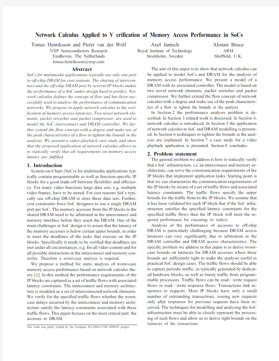
Network calculus is based on bounds of traffic flows.If a flow is bounded by a monotonously non-decreasing function b(?t)then the amount of traffic that flows through a given point in the network during any period of length ?t is smaller than or equal to b(?t).A useful family of functions for con-cise descriptions of bounds of traffic flows are so called (σ,ρ)functions,where ρis the average bandwidth and σlimits the burstiness of the flow. They have the form b(?t) =σ +ρ?t,(1)as illustrated in Figure 1.

A flow has a constant packet size L and the flow travels on a link with a capacity C.There is a lower limit for the bursti-ness because of the packet size:σ≥L (1-ρ/C).Based on the characterization of flows and the link capacity,Cruz has de-

rived formulas to compute upper bounds for worst-case de-lay,average delay and backlog for a variety of network elements such as constant delay line,regulator,and a number of different multiplexers.The definition of delay is the time from the first bit of a packet enters a network element until the first bit of the packet exits the network element.

Multiplexers are the most interesting and challenging net-work elements.A busy period is defined to be a maximal in-terval of time such that data flows on the output link of the multiplexer at rate C out throughout the interval.According to [1]no bit ever has to wait longer than the longest busy period in a multiplexer.With additional knowledge,the delay bound can be made tighter,e.g.a locally first-come-first-served (LFCFS)2-input multiplexer with C 1=C 2=C out =C has the worst-case delay (Equation 4.27 in [1]):

(2)

So far the network calculus theory has not been applied to analysis of memory access performance of SoCs.There are a number of characteristics in SoC architectures that are not easily taken into account by the network calculus theory.?Packets change size while travelling through an on-chip network.For instance a read-request packet is trans-formed into a burst of data by the memory.

?Most network calculus formulas assume that network elements process data when there are packets on the inputs.DRAMs however spend time on preparation and refresh activities although there are requests available.?The number of uncompleted transactions at a given time is often limited and can be statically determined in a SoC.This information can be used to derive signi?-cantly more realistic bounds on latency and buffer https://www.doczj.com/doc/e77535005.html,work calculus does not take this into account.

?SoC ?ows have speci?c latency constraints that can be exploited.Often,the delay of an individual transaction is less interesting than the worst-case aggregate delay of a number of transactions;e.g.in video processing the deadlines are attached to processing of an entire frame and not to individual read or write transactions.

These specific characteristics make it worthwhile to adapt network calculus for the SoC domain in order to derive tight-er bounds and avoid over-design of hardware resources.

5. SoC infrastructure model

Our contribution to the modelling of the SoC infrastruc-ture consists of two parts,two new network elements and a method to model a DRAM by making use of these two new network elements.

5.1 Packet stretcher and packet compressor

We introduce two novel network elements,packet stretch-er and packet compressor.These are used to model the re-quest to response transformations in memory transactions and the clock cycles that are spent on DRAM preparation.

Figure 1. (σ,ρ) bound on flow

length of period (?t)

amount of data σ+ρ?t

D 1σ2

C ρ2–---------------σ1C ρ1–---------------???

?ρ2C ρ2–---------------??

??+≤

A packet stretcher changes the size of a packet from L in to L out ,where L out >L in .The input link and the output link may have different capacities C in and C out .The bandwidth chang-es according to the packet stretching:ρout =(L out /L in )ρin .To compute the burstiness σout we need one definition.The earliest possible arrival time of packet p in a burst that starts with packet 1 at time 0 is:

a(p) = max{(p L in )/C in,((p L in )-σin )/ρin }- L in /C in (3)The burstiness of the output of the packet stretcher is:σout = max p {p L out -ρout (a(p)+L out /C out )}(4)It holds that σout ≤(L out /L in )σin .This is explained by the fact that the time for a packet after the stretcher is longer than the time for a packet before the stretcher, L in /C in ≤L out /C out .The delay of a packet stretcher is zero because the first bit of the output packet is sent at the same time as the first bit of the input packet arrives.The input packet inter-arrival time must be at least as long as the time it takes to send an output packet (L out /C out ).If the input packet inter-arrival time could be shorter,a regulator is needed in conjunction with the packet stretcher in the model,see Figure 2.A regulator in conjunction with a packet stretcher has ρq =(C out /L out )L in B/s and σq =L in (1-(C out L in )/(L out C in ))B.We have derived these characteristics directly from the fact that stretched packets should not overlap.We have further derived the maximum delay of the regulator as:

D = (C in σin /(C in -ρin )-σq )/ρq -σin /(C in -ρin )(5)This bound can be made tighter if the packet sizes are taken into account in a similar way as explained for multiplexers in Section 6.1.

A packet compressor changes the size from L in to L out ,where L out

5.2 DRAM model

The DRAM and the DRAM controller are modelled to-gether.The model is depicted in Figure 3for two flows.We model the multiplexing between requests as multiplexing be-tween abstract memory packets (AMPs).The AMPs have a size that corresponds to how much of the raw capacity of the DRAM interface they use in the worst case.An AMP ac-counts for the time the memory controller is occupied with the transaction.The size of the AMPs depends on the size

and alignment of transactions as well as the mapping of transactions to DRAM banks and the DRAM specification (DDR,DDR2,LPDDR,DDR3).If only long,well-aligned bursts that cyclically access all banks are used,the time for activating and precharging DRAM rows can be overlapped with data transfers and the AMPs do not include that time.

We assume that the write data is available when a corre-sponding write request is chosen by the multiplexer in the DRAM controller.In this way,the write data does not need to be modeled separately in the DRAM model.

The request flows (1R and 2R )are regulated and stretched into AMP flows (1M and 2M )on links with capacity equal to the raw DRAM interface capacity.The delay of the regula-tors in conjunction with the packet stretchers is denoted by D MR .The DRAM is modelled as a link with the raw capacity of the DRAM interface.The multiplexer thus has the same capacity on all input/output links.The delay in the multiplex-er in the DRAM controller is denoted by D MM .An additional flow of AMPs is introduced to model the refresh cycles of the DRAM (3M ).In the model the refresh generator is a pe-riodic source of AMPs.Some jitter is allowed on the refresh,so we assume that the refresh requests are multiplexed along with the normal requests before issued to the DRAM.

The multiplexer may use any arbitration policy.For exam-ple round-robin (RR)or fixed priority (FP)can be used.Equation (2)can be used to get an upper bound on D MM for those policies,but tighter bounds can be computed by mak-ing use of more information as shown in the next section.The AMPs are demultiplexed in the model to separate the response flows.The memory execution delay (D ME )is then modelled as a constant delay line with the delay equal to the worst-case delay of the DRAM.If the master waits for the first bits of the response packet (e.g.critical-word-first cache line refill),the delay to the first bits of the packet is modeled.If the master waits for the complete response packet the de-lay to the last bits of the packet is modeled.A packet com-pressor converts AMPs to response packets.

The total delay from the time when a request enters the DRAM controller until the response is available is:D M =D MR +D MM +D ME (6)

Figure 2. Regulator in conjunction with packet stretcher

(σ,ρ) regulator

Packet Stretcher out

in σin ,ρin , L in , C in

σq ,ρq , L q = L in , C q = C in

σout ,ρout , L out > L in , C out

Figure 3. DRAM model

(σ,ρ)PS

(σ,ρ)

PC PC

D ME1D ME2

(σ,ρ)=Regulator PS=Packet Stretcher PC=Packet Compressor R=Refresh Generator D=Constant Delay Line

Link that models DRAM interface raw capacity

In the actual hardware,no request regulators,packet stretch-ers,AMPs,or packet compressors are present.They are only present in the model.In the actual hardware,the requests are queued in the DRAM controller.

6. Tight bounds considerations

The modelling approach presented in the previous section makes it possible to compute latency bounds of SoC memory accesses.For SoC performance analysis it is however neces-sary to derive tight bounds.In this section we discuss how to tighten the bounds compared to network calculus theory by Cruz.This is done by a different analysis approach and by more accurate traffic descriptions.

6.1 Packet size and speci?c arbitration policy Equation(2)is valid for all LFCFS arbitration policies. Also the packet size is not included in the formula.It pro-vides an explicit and concise formula,but does not give tight bounds.We propose to make use of an iterative numerical method to derive the worst-case delays in a multiplexer.For the longest busy period(LBP)we compute the earliest arriv-al time of each packet according to Equation(3).Then the following procedure is repeated for every flow.We compute the latest possible service time of each packet according to the specific arbitration policy,the worst-case state of the ar-biter,and the service times of previously served packets in the LBP.The delay of each packet in the flow is obtained by subtracting the earliest arrival time from the latest possible service time.A maximum operation over the delays of all packets in the flow in the LBP gives the worst-case delay for the flow.

6.2 Degree

We introduce the degree of a flow as the maximum number of packets of a flow that are in flight at any point in time.This is used to limit the maximum backlog and to get tighter bounds on the total delay for consecutive transac-tions.A degree of1implies that a packet never has to wait for another packet of the same flow.This also means that the backlog in any network element is no more than 1 packet. The degree leads to later arrival times of packets because there is a dependency on the service time of previous pack-ets.Equation(3)is not applicable when the degree is taken into account.The arrival times are in this case computed with an iterative numerical method similar to the one explained in Section6.1 for service times.

6.3 Consecutive transactions

So far we have only discussed the analysis of the worst-case delay for a single transaction.In SoCs the worst-case aggregate delay of consecutive transactions is important,es-pecially for the read flows of programmable processors.The latency constraint is specified as the maximum aggregate de-lay for all transactions in a period?t.The straightforward way is to multiply the number of transactions with the max-imum delay per transaction.One way to tighten the bounds for a multiplexer is to make use of the degree.The read flows

of a programmable processor typically have a low degree.

For a flow with degree1we know that maximally one packet

of that flow waits for any packet of another flow in the case

of RR arbitration.The number of packets from each flow

during?t is limited by n i(?t)=ceil((σi+ρi?t)/L i).Consider N flows that are ordered in increasing n i.With RR arbitration

we get for flow k(with degree1)that the worst case aggre-

gate delay of the multiplexer is bounded by:

(7) 6.4 Peak characteristics

We introduce peak characteristics of?ows.Programmable

processors exhibit flows with bursty characteristics.When

such a flow is modelled withσandρ,σis large.This leads

to long worst-case delays in many network elements.By in-

troducing peak characteristics,σp andρp,a more accurate

bound on the traffic can be described.During a burst,the av-

erage bandwidth isρp,which is always larger than the long-

term average bandwidthρ,but smaller than the link capacity

C.The burstiness during a burst,σp,is thereby smaller than

the long-term burstinessσ.Typicallyρp andσp are chosen so

thatσp = L (1-ρp/C), the minimum possible burstiness.

The amount of data in a flow during any period of time of

length?t is bounded according to Equation(1).If we know

C the bound can be restricted to b(?t)=min{C?t,σ+ρ?t}.

With the peak characteristics(σp,ρp)it can be further re-

stricted,b(?t)=min{C?t,σ+ρ?t,σp+ρp?t},see Figure4. The bound b(?t)is the thick line.This can be generalized to any number of(σi,ρi)pairs to describe the traffic.If more(σi,ρi)pairs are used,tighter bounds can be derived,but the anal-ysis becomes more cumbersome.For the arrival time calcu-lation of every packet all(σi, ρi) pairs have to be checked.

7. Case study

A video playback application has been studied to validate the usefulness of the presented theory.The video playback application is implemented on a shared memory architecture.

7.1 Case study description

The processors and hardware IP use the AXI interface pro-tocol[8]to access DRAM.There are four processing ele-ments(PEs),two programmable processors,an ARM CPU and a TriMedia DSP,and two hardware IPs,a scaler and a display controller(DC).A block diagram is shown in Figure5.All communication between the PEs goes via shared memory.The ARM reads a bitstream from the flash D k aggregate

n i

L i

C----

–

∑n k L i C----

i k

∑

≤

Figure 4. Peak characteristics

length of period

σ+ρ?t

σp+ρp?t

C?t

σp

memory (not shown in Figure 5),demultiplexes the bit-stream into video and audio and handles the audio decoding.The video bitstream is written into DRAM.The TriMedia runs a video decoder that reads the bitstream and decodes it into raw video frames of size 720x576@50frames per sec-ond in 8bit YUV4:2:0video format (1.5bytes/pixel).The scaler reads the raw video from DRAM,scales the video to the display size (800x600),converts the video format into 32bit RGB,and writes the scaled and converted video data back into DRAM.The DC reads the video from the DRAM and sends it to the display.The frame rate is 50frames per second in all the steps.

There are 7request flows in the case study.The ARM reads (1)and writes (2),the TriMedia reads (3)and writes (4),the scaler reads (5)and writes (6),and the DC reads (7).In the ARM and TriMedia read flows,both instructions and data reads are included.The characteristics are given in Table 1. The packet size is L=n R B for all request flows.In this case study,the ρand σof the flows from the ARM and the TriMedia are estimated based on clock frequency,cache miss rates,and basic characteristics of bitstream de-multiplexing and video decoding.The ρand σof the flows from the scaler and the DC are calculated based on frame rate,resolution,and pixel formats.The flows from the scaler and the DC are strictly periodic,so that σ=L (1-ρ/C).The transaction sizes (TS)are derived from cache line sizes from the programmable processors and sizes of the local memo-ries in the hardware IPs.

The degree of flows 1and 3is 1because only one transac-tion is busy at any point in time.Flow 4R has σp =0.99n R B,ρp =n R MB/s.This is based on the assumption that the copy back unit of the data cache is regulated to write maximally one cache line per 1μs.

The latency constraints (LC)on the read flows for the

ARM and the TriMedia are derived from allowed stall cycles to be able to finish the processing on time.The LC on the read flows from the scaler and the display controller are de-rived from the sizes of local memories in the HW IPs.The LC on the write flows are derived from the bandwidth,the sizes of the write back buffer memories and the implementa-tion of the synchronization scheme.The LC are given in Table 1.Window refers to a time window,a ‘1’indicates that the requirement holds per transaction.The type can be round-trip latency (round) or one-way latency (one).

The SoC AXI interconnect runs at 100MHz and has 8byte wide data connections.The DRAM controller runs also at 100MHz and uses a 4byte wide DDR interface (raw capacity is 800MB/s).The request connections run at 100MHz and are wide enough to transfer one request per clock cycle.All four PEs have private AXI channels to the memory controller.In AXI,read requests and write requests are independent,so each flow has its own channel to the DRAM controller.There is thus only one single point of ar-bitration in the system.Round robin (RR)is used as arbitra-tion policy.It takes two clock cycles (20ns)for a request to travel from a PE to the memory controller and it also takes two clock cycles for a response to travel from the memory controller back to the PE.

A 128byte AXI transaction is split up into four DRAM bursts.The AXI transactions are issued on aligned addresses so that all DRAM bursts from one AXI transaction reside in the same DRAM row.This means that precharge and acti-vate is not needed in the middle of one AXI transaction.From the DRAM specification [9]we can compute that a 128

B read transaction including activate and following pre-charge keeps the memory controller busy for 22cycles.Sim-ilar calculations for 32B read gives 10cycles,for 32B write 13 cycles, and for 128B write 25 cycles.

7.2 Modelling and results

The DRAM is modelled according to Section 5.2.A 128B read request is stretched to an AMP of size 22x 8B =176B.A 128B write request is stretched to a 200B AMP,a 32B read request is stretched to a 80B AMP,a 32B write request is stretched to a 104B AMP,and the refresh generator gen-erates AMPs of 80B because a refresh takes 10cycles.In the case study,the request regulator is only applicable for flow 2because no other flows allow requests close to each other.For flows 1and 3that is guaranteed by the degree and for flow 4 it is guaranteed by the peak characteristics.

The request regulator for flow 2has the following D MR and other parameters:L out =104B,ρin =31250n R B/s,σin =2n R B,ρq =7692307n R B/s,σq =0.9231n R ,and D MR =120ns according to Equation (5)and the other for-mulas presented in Section 5.1.

The characteristics of the AMP flows at the memory mul-tiplexer,after request regulation and stretching,are comput-

Table 1. Flow characteristics and latency constraints Flow Type σ [B]ρ [kB/s]TS [B]LC window type 1R Read 4n R 189.9n R 326.00 ms 20 ms round 2R Write 2n R 31.25n R 32 3.00μs 1one 3R Read 4n R 320n R 1288.00 ms 20 ms round 4R Write 18.4n R 243n R 128 3.00μs 1one 5R Read 0.99n R 243n R 128 4.11μs 1round 6R Write 0.99n R 750n R 128 3.00μs 1one 7R

Read

0.99n R 750n R 128 2.66μs 1round

ARM CPU TriMedia DSP Scaler Display controller

SoC

DRAM

Cmd generation R

W R

Refresh

Figure 5. Block diagram of case study SoC+DRAM

DRAM controller

ed from the sizes of the AMPs and the characteristics of the request flows according to the formulas in Section5.1.The flows are described in Table2.Flow8models refresh.Addi-tional information is that flows1M and3M have degree1and flow 4M hasσp = 150 B,ρp = 200 MB/s.

The memory multiplexer delay accounts for the largest share of the transaction delays.Because all links have the same capacity,and RR is an LFCFS policy,Equation(2)ex-tended to 8flows can be used.That gives the bounds in the second column in Table3,which are not within the require-ments.Tighter bounds are derived according to Section6.1. The numbers from that analysis are shown in the third col-umn in Table3.Also those bounds are not within the re-quirements.Even tighter bounds can be given by including the peak characteristics of flow4and the degree of flows1 and3as described in Section6.2and Section6.4.Those bounds are shown in the fourth column in Table3.E.g.for flow2,the second packet can arrive at130ns after the start of the LBP.In the worst case it is serviced2530ns after the start of the LBP. The delay is thus 2530-130=2400 ns.

The total transaction delays consist of the wire delays and the memory delays.The memory execution delays(D ME)are determined according to Section5.2.Flow1uses critical word first,all the others do not.D MR and D MM have been presented above.The worst case transaction delays D total are presented in column 5 in Table3.

Flows1and3have constraints for the aggregate delay of the transactions within a20ms time window.As explained in Section6.3a straightforward bound on consecutive trans-actions is to multiply the number of transactions with the de-lay per transaction.E.g.for flow3there can be6404 transaction with a delay of1520ns,which gives an aggregate delay of9.73ms.This does not meet the latency constraint for flow3.By making use of Equation(7)the aggregate de-lay for flow3can be limited to627*1520ns+1934*1390ns +1241*1290ns+1059*1190ns+18*970ns+ 1525*680ns=7.56ms.This meets the latency constraint for flow 3.

8. Discussion and Conclusions

We have shown how network calculus can be applied to the performance analysis of SoC memory accesses.We fo-cused on DRAM accesses because they are the most chal-lenging.The approach we have taken is also applicable to on-chip and off-chip SRAMs and memory mapped registers. The challenge is to derive tight bounds with concise mod-els and simple analysis.There is a trade-off between tight-ness and simplicity.We have added information in the form of arbitration policy,degree,and peak characteristics to the basic(σ,ρ)traffic descriptions to improve the tightness.This tightens the bounds significantly at an acceptable modelling and analysis effort.For the presented case study all the pre-sented techniques were needed to show that the design fulfils all requirements.

We conclude that it is possible to apply network calculus for worst-case analysis of memory access performance in https://www.doczj.com/doc/e77535005.html,ing the presented modelling approach and tight analysis considerations,sufficiently tight bounds can be de-rived.Future work is to include this analysis approach in a system performance verification environment. References

[1]R.L.Cruz.A Calculus for Network Delay,Part I:Network El-

ements in Isolation and part II:Network Analysis.In IEEE Transactions on Information Theory,vol.37,no.1,pp.114-141, January 1991.

[2]https://www.doczj.com/doc/e77535005.html,work Calculus.Springer Verlag,no.2050,

LCNS, 2001.

[3]D.Stiliadis and https://www.doczj.com/doc/e77535005.html,tency-Rate Servers:A General

Model for Analysis of Traffic Scheduling Algorithms.IEEE/ ACM Transactions on Networking,vol.6,no.5,pp.611-624, October 1998.

[4]L.Thiele,S.Chakraborty,and M.Naedele.Real-time calculus

for scheduling hard real-time systems.Proc.of the Internation-al Symposium on Circuits and Systems(ISCAS),pp.101-104, vol. 4, 2000.

[5]M.Jersak et al.Performance Analysis for Complex Embedded

Applications.International Journal of Embedded Systems,Spe-cial Issue on Codesign for SoC,vol.45,issue1/2,pp.33-49, 2005.

[6]Y.-T.S.Li et al.Performance Estimation of Embedded Soft-

ware with Instruction Cache Modeling.IEEE pp.380-387,1995.

[7]J.Staschulat et al.Analysis of Memory Latencies in Multi-

Processor Systems. Workshop on WCET, pp. 33-36, 2005. [8]AMBA3Specification&Assertions.https://www.doczj.com/doc/e77535005.html,/

products/solutions/axi_spec.html

[9]Micron,Mobile DDR SDRAM MT46H16M32LF.http://

https://www.doczj.com/doc/e77535005.html,/pdf/datasheets/dram/mobile/

MT46H32M16LF.pdf

Table 2. AMP ?ow characteristics

Flowσ [B]ρ [MB/s]L [B]

1M318.615.19280 2M207.6 3.250104 3M692.256.320176 4M3670.148.600200 5M167.042.768176 6M162.5150.000200 7M148.3132.000176 8M79.010.24080

Table 3. Delays per request [ns]

Flow Equation (2)RR Peak and degree D total 114872456013901490 215531240024002640 312884386012701520 49678544014901720 513970127012701520 610902124012401470 711337127012701520 815378139013901490

一节课微积分入门

一节课微积分入门 “一节课微积分入门”原本是笔者制作的一个教学视频，在酷6网上点击率一度突破12万（可惜现在删了，但土豆网上还有），而大学教授的同类视频，点击率最高才2千多。笔者身边好几个学不懂微积分的人都在里面受益。这是笔者独创的一套最简捷，清晰，易懂的教学方法，从零开始，在短短的 40分钟内，让大家理解：微积分最基本的原理，牛莱公式的本质含义和基本求导方法。希望能在微积分教学的历史长河中留下一朵小小的浪花。考虑到很多朋友不喜欢看教学视频，而更喜欢阅读文档，笔者把最基本的教学思路整理下来，供大家学习和参考，（看不懂的可以网上搜视频做为辅助学习）目录： 1巧妙的叠加方法 2问题的提出：求y=x2曲线围成的面积 3切割法求出近似面积 4寻找“远房表叔”来帮忙 5对“远房表叔”进行切割和叠加 6“表叔”和“表侄”的一一对应。 7一一对应关系式的提出 8一一对应关系式的进一步表达：牛莱公式 9一一对应关系式的变形：导函数的定义 10求导的2个例题 11导函数的意义

1巧妙的叠加方法方法一非常麻烦，要测1千次，再加1千次，方法二就简单多了，因为反正不需要知道每个小棍子的长度，只测一次就够了。这就是“叠加法”，在后面的微积分学习中，我们会非常巧妙的用到“叠加法”。 2 问题的提出：求y=x2曲线围成的面积

这种曲线围成的面积，显然用初等数学无法解决，这就需要我们巧妙构思，另辟蹊径了。 3 切割法求出近似面积我们把横坐标切成1000份，然后切割出999个小长方形，每个小长方形的宽都是1/1000，小长方形的长则是该点对应的函数值，这样每个小长方形的面积都可以求出来了。

大一上学期微积分期末试卷及答案

1 1?设f(x) 2cosx,g(x) (l)sinx在区间(0, —)内( 2 2 A f (x)是增函数，g (x)是减函数 Bf (x)是减函数，g(x)是增函数 C二者都是增函数 D二者都是减函数2、x 0时，e2x cosx与sinx相比是() A高阶无穷小E低阶无穷小C等价无穷小 1 3、x = 0 是函数y = (1 -sinx)书勺() A连续点E可去间断点C跳跃间断点 4、下列数列有极限并且极限为1的选项为( ) n 1 n A X n ( 1) B X n sin - n 2 1 1 C X n n (a 1) D X n cos— a n 5、若f "(x)在X。处取得最大值，则必有() A f /(X。)o Bf /(X。)o Cf /(X。)0且f''( X o)

5、若则a,b 的值分别为： X 1 X + 2x-3

2 1 In x 1 ; 2 y x 3 2x 2; 3 y log^x 1 -,(0,1), R ; 4(0,0) x lim 5解：原式=x 1 (x 1)( x m ) ~~1)( x 7 b lim 3) x 7, a 1、 2、、判断题无穷多个无穷小的和是无穷小( lim 沁在区间(， X 0 X 是连续函数() 3、 f"(x 0)=0—定为f(x)的拐点 () 4、若f(X)在X o 处取得极值，则必有 f(x)在X o 处连续不可导( 5、 f (x) 0,1 f '(x) 0令 A f'(0), f '(1),C f (1) f (0),则必有 A>B>C( 1~5 FFFFT 二、计算题 1用洛必达法则求极限 1 2 ~ lim x e x x 0 1 e 解：原式=lim x 0 1 x x 2 lim e x 2 ( 2x x 0 2x 3 3 4 k 2 若 f(x) (x 10),求f”(0) 3) 1 lim e x x 0 3 3 2 2 f '(x) 4(x 10) 3x 12x (x 3 3 2 3 2 2 f ''(x) 24x (x 10) 12x 3 (x 10) 3x 24x f ''(x) 0 10)3 3 .. .3 3 4 , 3 (x 10) 108 x (x 10)2 4 r t I 八］ 2 3 求极限 lim(cos x)x x 0

微积分在生活中的应用

龙源期刊网 https://www.doczj.com/doc/e77535005.html, 微积分在生活中的应用作者：曹红亚来源：《数学大世界·中旬刊》2020年第01期【摘要】微积分产生于十七世纪后期，完善于十九世纪。在现代社会中，微积分是高等数学中至关重要的组成部分，在数学领域中扮演着不可替代的角色，与此同时，微积分在现实生活中的应用也越来越广泛。本文将就微积分在生活中的应用进行深入的分析与探究。【关键词】微积分;现实生活;实际应用众所周知，微积分建立的基础是实数、函数以及极限。关于微积分的定义，其指的是微分学和积分学二者的总称，其更代表着一种数学思想。微积分的发展与现实生活的发展是密切相关的，现在的微积分已经广泛存在于诸多自然科学当中，如天文学、生物学、工程学以及经济学等等，在现实生活着发挥着越来越重要的作用。以下笔者结合自己多年的相关实践经验，就此议题提出自己的几点看法和建议。一、微积分在日常工作中的应用微积分不仅仅应用在科研领域，其更实实在在地存在于我们的生活当中。例如日常生活中，我们需要装修或者从事装修工作，都需要进行工程预算，这时我们便会不自觉地应用微积分原理，首先将整个装修工程科学划分成为多个小单元，然后对应用到的材料和工时进行计算，最终得出总的造价。再比如，现在很多人特别是年轻人都希望创造一份属于自己的事业，那么其在创业时可能会应用到微积分。如对所选地址处的车流量以及人流量进行了解，在一天的几个时间段，做一分钟的调查，测出经过的人数或车数，再通过计算得出每天或每月的人流量或车流量，这将是我们创业的一个重要参考面。二、微积分在曲线领域中的应用在微积分的现实应用中，最具代表性的便是求曲线的长度、切线以及不规则图形的面积。如在当前社会中，相关数字音像制品或者正流行的数字油画，其都需要将图像和声音分解成为一个个像素或者音频，利用数字的方式来进行记录、完成保存。在重放的时候，再由设备用数字方式来解读还原，使我们听到或看到几乎和原作一模一样的音像。再比如，中央电视台新闻频道的时事报道中常看到地球转向某一点，放大，现出地名，播送最新动态的新闻画面。它的整体概貌是拼装的，是由卫星将地球分成一个个小区域进行拍照，最后拼接成地球的形状，才让我们形象地、跨时空地欣赏新闻报道的同步魅力。三、微积分在买卖中的应用

同济大学高等数学1期末试题(含答案)

1. 若82lim =?? ? ??--∞→x x a x a x ，则_______.2ln 3- 2. =+++→)1ln()cos 1(1 cos sin 3lim 20x x x x x x ____.2 3 3.设函数)(x y y =由方程4ln 2y x xy =+所确定，则曲线)(x y y =在)1,1(处的切线方程为________.y x = 4. =-++∞→))1(sin 2sin (sin 1lim n n n n n n πππ Λ______.π2 5. x e y y -=-'的通解是____.x x e e y --=21C 二、选择题（每题4分） 1.设函数)(x f 在),(b a 内连续且可导，并有)()(b f a f =，则（D ） A ．一定存在),(b a ∈ξ，使 0)(='ξf . B. 一定不存在),(b a ∈ξ，使 0)(='ξf . C. 存在唯一),(b a ∈ξ，使 0)(='ξf . D.A 、B 、C 均不对. 2.设函数)(x f y =二阶可导，且 ,)(),()(,0)(,0)(x x f dy x f x x f y x f x f ?'=-?+=?<''<'，当,0>?x 时，有（A ） A. ,0<>?dy y C. ,0?>y dy 3. =+?-dx e x x x ||2 2)|(|(C) A. ,0B. ,2C. ,222+e D. 26e 4. )3)(1()(--=x x x x f 与x 轴所围图形的面积是（B ） A. dx x f ?3 0)( B. dx x f dx x f ??-3110)()( C. dx x f ?-30)( D. dx x f dx x f ??+-3110)()( 5.函数Cx x y +=361 ，（其中C 为任意常数）是微分方程x y =''的（C ） A ．通解B.特解C.是解但非通解也非特解D.不是解

微积分练习题及解析

练习题 1、质量为2kg 的某物体在平面直角坐标系中运动，已知其x 轴上的坐标为x=3+5cos2t ，y 轴上的坐标为y=-4+5sin2t ，t 为时间物理量，问： ⑴物体的速度是多少？ ()'10sin(2)x dx V x t t dt = ==- ()'10cos(2)y dy V y t t dt === 2210x y V V V =+= ⑵物体所受的合外力是多少? 222(3)(4)5x y -+-= 运动轨迹是圆，半径为5，所以是做匀速圆周运动 22*100405 mv F N r === ⑶该物体做什么样的运动？匀速圆周运动 ⑷能否找出该物体运动的特征物理量吗？圆心（3,4），半径5 2、一质点在某水平力F 的作用下做直线运动，该力做功W 与位移x 的关系为W=3x-2x 2,试问当位移x 为多少时F 变为零。 34dW F x dx = =-，所以当x=3/4时，F=0 3、已知在距离点电荷Q 为r 处Ａ点的场强大小为E= KQ r 2, 请验证Ａ点处的电势公式为：U = KQ r 。规定无穷远处电势为零，A 处的电势即为把单位正电荷缓慢的从无穷远处移到A 点所做的功我们认为在r 变化dr 时，库仑力F 是不变的，则2 kQq dW F dr dr r =-?=- ? 所以2 0W r kQq dW dr r ∞=-?? 即21r q kQq dr r ?∞=? 所以1|r kQ kQ r r ?∞=-=

4、某复合材料制成的一细杆OP 长为L ，其质量分布不均匀。在杆上距离O 端点为x 处取点A ，令M 为细杆上OA 段的质量。已知M 为x 的函数，函数关系为M=kx 2，现定义线密度ρ=dM dx ,问当x=L 2 处B 点的线密度为何？ 2dM kx dx ρ= = ,2L x kL ρ∴== 5、某弹簧振子的总能量为2×10-5J ，当振动物体离开平衡位置12 振幅处，其势能E P =，动能E k =。首先推导弹簧的弹性势能公式，设弹簧劲度系数为k ，伸长量为x 时的势能为E （x ）弹簧所具有的弹性势能即为将弹簧从原长拉长x 时所做的功 dW F dx kx dx =?=? 00W x dW kx dx ∴=??? 2 ()2 kx E x ∴= 所以在距平衡位置12振幅处的弹性势能为总能量的14 ，即655*10, 1.5*10p k E J E J --== 6、取无穷远处电势为零。若将对电容器充电等效成把电荷从无穷远处移到电容器极板上，试问，用电压U 对电容为C 的电容器充电，电容器存储的电能为何？开始时电容器存放的电荷量为零。 0022 1122q q E Q q q dE dQ U Q dE dQ C Q E CU C =?∴=∴==?? 7、在光滑的平行导轨的右端连接一阻值为R 的电阻，导轨宽度为L ，整个导轨水平放置在方向竖直向下的磁场中，磁场的磁感应强度为B 。有一导体棒ab 垂直轨杆并停放在导轨上，导体棒与导轨有良好的接触。在t=0时刻，给导

大一微积分期末试卷及答案

微积分期末试卷选择题（6×２） cos sin 1.()2 ,()()22 ()()B ()()D x x f x g x f x g x f x g x C π ==1设在区间（0，）内（　）。Ａ是增函数，是减函数是减函数，是增函数二者都是增函数二者都是减函数 2x 1 n n n n 20cos sin 1n A X (1) B X sin 21C X (1) x n e x x n a D a π→-=--== >、x 时，与相比是（　）Ａ高阶无穷小Ｂ低阶无穷小Ｃ等价无穷小Ｄ同阶但不等价无价小３、ｘ=０是函数ｙ=（１-sinx)的（　）Ａ连续点Ｂ可去间断点Ｃ跳跃间断点Ｄ无穷型间断点４、下列数列有极限并且极限为１的选项为（）n 1 X cos n = 2 00000001() 5"()() ()()0''( )<0 D ''()'()0 6x f x X X o B X o C X X X X y xe =<===、若在处取得最大值，则必有（　）Ａf ＇f ＇f ＇且f f 不存在或f 、曲线（）Ａ仅有水平渐近线Ｂ仅有铅直渐近线Ｃ既有铅直又有水平渐近线Ｄ既有铅直渐近线 1~6 DDBDBD 一、填空题 1d 12lim 2,,x d x ax b a b →++=ｘｘ２２１１、（）＝ｘ+1 、求过点（２，０）的一条直线，使它与曲线ｙ＝相切。这条直线方程为：ｘ２３、函数ｙ＝的反函数及其定义域与值域分别是：２＋１４、ｙ拐点为：ｘ５、若则的值分别为：ｘ＋2x-3

1 In 1x + ; 2 322y x x =-; 3 2 log ,(0,1),1x y R x =-; 4(0,0) 5解：原式=11 (1)() 1m lim lim 2 (1)(3) 3 4 77,6 x x x x m x m x x x m b a →→-+++== =-++∴=∴=-= 二、判断题 1、无穷多个无穷小的和是无穷小（） 2、 0 sin lim x x x →-∞+∞在区间（，）是连续函数（） 3、 0f"(x ）=0一定为f(x)的拐点（） 4、若f(X)在0x 处取得极值，则必有f(x)在0x 处连续不可导（） 5、设函数ｆ(x)在 [] 0,1上二阶可导且 ' ()0A ' B ' (f x f f C f f <===-令（），则必有 1~5 FFFFT 三、计算题 1用洛必达法则求极限2 1 2 lim x x x e → 解：原式=2 2 2 1 1 1 3 3 2 (2)lim lim lim 12x x x x x x e e x e x x --→→→-===+∞- 2 若3 4 ()(10),''(0)f x x f =+求解：3 3 2 2 3 3 3 3 2 3 2 2 3 3 4 3 2 '()4(10)312(10) ''()24(10)123(10)324(10)108(10)''()0 f x x x x x f x x x x x x x x x x f x =+?=+=?++??+?=?+++∴= 3 2 4 lim (cos )x x x →求极限

微积分在生活中的应用Word版

微积分在生活中的应用（何杰东陈新亮连冠才施楠信工一班北二830）一.摘要牛顿、莱布尼兹发明微积分以后，人们才有能力把握运动和过程。有了微积分，就有了工业革命，就有了大工业生产，也就有了现代化的社会。航天飞机、宇宙飞船等现代化交通工具都是在微积分的帮助下制造出来的。微积分在人类社会从农业文明跨入工业文明的过程中起到了决定性的作用。微积分是为了解决变量的瞬时变化率而存在的。从数学的角度讲，是研究变量在函数中的作用。从物理的角度讲，是为了解决长期困扰人们的关于速度与加速度的定义的问题。“变”这个字是微积分最大的奥义。因此，了解微积分在生活中的应用对于我们解决实际问题有很大的帮助。二．关键词：物理，经济，应用。三．引言：通过研究微积分在物理，经济等方面的具体应用，得到微积分在现实生活中的重要意义，从而能够利用微积分这一数学工具科学地解决问题。获取资料的途径主要是互联网。四（一）在物理中的应用例1，研究物体做匀变速直线运动位移问题时；对于匀速直线运动，位移和速度之间的关系我们都清楚,x=vt，但如果物体的速度大小时刻发生变化，那么物体的位移如何求解呢？此时，微积分就成了我们有利工具。我们可以把物体运动的时间无限细分。在每一份时间内，速度的变化量非常小，可以忽略这种微小变化，认为物体在做匀速直线运动，因此根据已有知识位移可求；接下来把所有时间内的位移相加，即“无限求和”，则总的位移可以知道。现在我们明白，物体在变速直线运动时候的位移等于速度时间图像与时间轴所围图形的面积；例2，研究匀速圆周向心加速度的方向问题时；根据牛顿第二定律，我们可以知道匀速圆周运动加速度的方向指向圆心；同时利用极限思想，也可以加速度的方向。当圆周上的两个点无限靠近时，速度变化量也无限的小，因此由VAVB△V围成的等腰三角形的底角接近90，因此速度变化量和速度垂直，而速度又和半径垂直，因此，匀变速圆周运动中，加速度的方向始终指向圆心。例3.研究变力做功问题时；对于恒力做功，我们可以利用公式直接求出；但对于变力，我们不能利用公式；这种情况下，我们要借助于微积分，我们可以把位移无限细分，在每一个小位移上，力的变化很小，可以看作是恒力，根据公式算出力所作的功；然后把每一个小位移上的功无限求和，那么就可以求出变力做的总功是多少。（二）在经济上的应用 1.1 边际分析在经济分析中的的应用 1.1.1 边际需求与边际供给设需求函数Q=f（p）在点p处可导（其中Q为需求量，P为商品价格），

微积分下册期末试卷附答案

中南民族大学06、07微积分（下）试卷及参考答案 06年A 卷评分阅卷人 1、已知22 (,)y f x y x y x +=-,则=),(y x f _____________. 2、已知,则= ?∞ +--dx e x x 0 21 ___________. π =? ∞ +∞ --dx e x 2 3、函数 22 (,)1f x y x xy y y =++-+在__________点取得极值. 4、已知y y x x y x f arctan )arctan (),(++=,则= ')0,1(x f ________. 5、以x e x C C y 321)(+=(21,C C 为任意常数)为通解的微分方程是 ____________________. 二、选择题(每小题3分,共15分) 评分阅卷人 6 知dx e x p ?∞ +- 0 )1(与?-e p x x dx 1 1 ln 均收敛, 则常数p 的取值范围是( ). (A) 1p > (B) 1p < (C) 12p << (D) 2p >

7 数???? ?=+≠++=0 ,0 0 ,4),(222 22 2y x y x y x x y x f 在原点间断, 是因为该函数( ). (A) 在原点无定义 (B) 在原点二重极限不存在 (C) 在原点有二重极限,但无定义 (D) 在原点二重极限存在,但不等于函数值 8、若 2 2223 11 1x y I x y dxdy +≤= --?? ,22223212 1x y I x y dxdy ≤+≤=--??, 2 2223 324 1x y I x y dxdy ≤+≤=--?? ,则下列关系式成立的是( ). (A) 123I I I >> (B) 213I I I >> (C) 123I I I << (D) 213I I I << 9、方程x e x y y y 3)1(596+=+'-''具有特解( ). (A) b ax y += (B) x e b ax y 3)(+= (C) x e bx ax y 32)(+= (D) x e bx ax y 323)(+= 10、设∑∞ =12n n a 收敛，则∑∞ =-1) 1(n n n a ( ). (A) 绝对收敛 (B) 条件收敛 (C) 发散 (D) 不定三、计算题(每小题6分,共60分) 评分评分评阅人 11、求由2 3x y =,4=x ,0=y 所围图形绕y 轴旋转的旋转体的体积.

微积分中10大经典问题

微积分中10大经典问题最初的想法来自大一，当时想效仿100个初等数学问题，整理出100个经典的高等数学问题（这里高等数学按广义理解）。可惜的是3年多过去了，整理出的问题不足半百。再用经典这把尺子一量，又扣去了一半。这里入选原则是必须配得起“经典”二字。知识范围要求不超过大二数学系水平，尽量限制在实数范围内，避免与课本内容重复。排名不分先后。 1）开普勒定律与万有引力定律互推。绝对经典的问题，是数学在实际应用中的光辉典范，其对奠定数学科学女皇的地位起着重要作用。大家不妨试试，用不着太多的专业知识，不过很有挑战性。重温下牛顿当年曾经做过的事，找找当牛人的感觉吧，这个问题是锻炼数学能力的好题！ 2）最速降线问题。该问题是变分法中的经典问题，不少科普书上也有该问题。答案是摆线（又称悬轮线），关于摆线还有不少奇妙的性质，如等时性。其解答一般变分书上均有。本问题的数学模型不难建立，即寻找某个函数，它使得某个积分取最小值。这个问题往深层次发展将进入泛函领域，什么是泛函呢？不好说，一个通俗的解释是“函数的函数”，即“定义域”不是区间，而是“一堆”函数。最速降线问题通过引入光的折射定律可以直接化为常微分方程，大大简化了求解过程。不过变分法是对这类问题的一般方法，尤其在力学中应用甚广。 3）曲线长度和曲面面积问题。一条封闭曲线，所围面积是有限的，但其周长却可以是无限的，比如02年高中数学联赛第14题就是这样一条著名曲线-----雪花曲线。如果限制曲线是可微的，通过引入内折线并定义其上确界为曲线长度。但把这个方法搬到曲面上却出了问题，即不能用曲面的内折面的上确界来定义曲面面积。德国数学家H.A.Schwarz举出一个反例，说明即使像直圆柱面这样的简单的曲面，也可以具有面积任意大的内接折面。 4）处处连续处处不可导的函数。长久以来，人们一直以为连续函数除了有限个或可数无穷个点外是可导的。但是，魏尔斯特拉斯给出了一个函数表达式，该函数处处连续却处处不可导。这个例子是用函数级数形式给出的，后来不少人仿照这种构造方式给出了许多连续不可导的函数。现在教材中举的一般是范德瓦尔登构造的比较简单的例子。至于魏尔斯特拉斯那个例子，可以在齐民友的《重温微积分》中找到证明。其实上面那个雪花曲线也是一条处处连续处处不可导的曲线。

大一微积分期末试题附答案

微积分期末试卷一、选择题（6×２） cos sin 1.()2,()()22 ()()B ()()D x x f x g x f x g x f x g x C π ==1设在区间（0，）内（　）。Ａ是增函数，是减函数是减函数，是增函数二者都是增函数二者都是减函数 2x 1 n n n n 20cos sin 1n A X (1) B X sin 21C X (1) x n e x x n a D a π →-=--==>、x 时，与相比是（　）Ａ高阶无穷小Ｂ低阶无穷小Ｃ等价无穷小Ｄ同阶但不等价无价小３、ｘ=０是函数ｙ=（１-sinx)的（　）Ａ连续点Ｂ可去间断点Ｃ跳跃间断点Ｄ无穷型间断点４、下列数列有极限并且极限为１的选项为（）n 1 X cos n = 2 00000001 () 5"()() ()()0''( )<0 D ''()'()06x f x X X o B X o C X X X X y xe =<===、若在处取得最大值，则必有（　）Ａf ＇f ＇f ＇且f f 不存在或f 、曲线（）Ａ仅有水平渐近线Ｂ仅有铅直渐近线Ｃ既有铅直又有水平渐近线Ｄ既有铅直渐近线二、填空题 1 d 1 2lim 2,,x d x ax b a b →++=ｘｘ２２１１、（）＝ｘ+1 、求过点（２，０）的一条直线，使它与曲线ｙ＝相切。这条直线方程为：ｘ２３、函数ｙ＝的反函数及其定义域与值域分别是：２＋１ｘ５、若则的值分别为：ｘ＋2x-3

三、判断题 1、无穷多个无穷小的和是无穷小（） 2、 0sin lim x x x →-∞+∞在区间（，）是连续函数（） 3、 0f"(x ）=0一定为f(x)的拐点（） 4、若f(X)在0x 处取得极值，则必有f(x)在0x 处连续不可导（） 5、设函数ｆ (x) 在 [] 0,1上二阶可导且 '()0A '0B '(1),(1)(0),A>B>C( )f x f f C f f <===-令（），则必有四、计算题 1用洛必达法则求极限2 1 2 lim x x x e → 2 若34()(10),''(0)f x x f =+求 3 2 4 lim(cos )x x x →求极限 4 (3y x =-求 5 3tan xdx ? 五、证明题。 1、证明方程3 10x x +-=有且仅有一正实根。 2、arcsin arccos 1x 12 x x π +=-≤≤证明（）六、应用题 1、描绘下列函数的图形 21y x x =+

微积分在现实中的应用

微积分的应用微积分是研究函数的微分、积分以及有关概念和应用的数学分支。微积分是建立在实数、函数和极限的基础上的。微积分学是微分学和积分学的总称。它是一种数学思想，‘无限细分’就是微分，‘无限求和’就是积分。无限就是极限，极限的思想是微积分的基础，它是用一种运动的思想看待问题。微积分最重要的思想就是用"微元"与"无限逼近",好像一个事物始终在变化你不好研究,但通过微元分割成一小块一小块,那就可以认为是常量处理,最终加起来就行。微积分是与实际应用联系着发展起来的，它在天文学、力学、化学、生物学、工程学、经济学等自然科学、社会科学及应用科学等多个分支中，有越来越广泛的应用。特别是计算机的发明更有助于这些应用的不断发展。客观世界的一切事物，小至粒子，大至宇宙，始终都在运动和变化着。因此在数学中引入了变量的概念后，就有可能把运动现象用数学来加以描述了。微积分建立之初的应用：第一类是研究运动的时候直接出现的，也就是求即时速度的问题。第二类问题是求曲线的切线的问题。第三类问题是求函数的最大值和最小值问题。第四类问题是求曲线长、曲线围成的面积、曲面围成的体积、物体的重心、一个体积相当大的物体作用于另一物体上的引力。微积分学极大的推动了数学的发展，同时也极大的推动了天文学、力学、物理学、化学、生物学、工程学、经济学等自然科学、社会科学及应用科学各个分支中的发展。并在这些学科中有越来越广泛

的应用，特别是计算机的出现更有助于这些应用的不断发展。微积分作为一种实用性很强的数学方法和根据，在数学发展中的地位是十分重要的。例如，微分可以解决近似计算问题。比如：求sin29°的近似值，求不规则图形面积或几何体体积的近似值等。通过微积分求极限、利用微分中值定理，能够及时的放缩多项式，有利于不等式的化简和证明。极限求和、导数求和、积分求和也都是解决求数列前n项和的好方法。其次，数理化不分家。而且微积分在不等式中也有很大的运用，我们可以运用微积分中值定理，泰勒公式，函数的单调性，极值，最值，凸函数法等来证明不等式。在物理问题上，通过解微分方程研究物体运动问题、气体问题、电路问题也是非常普遍的。已知位移——时间函数计算速度，已知速度——时间函数计算加速度（即生活中交通管理方面的应用）；运动学中的曲线轨迹求解（即生活中在篮球投篮训练中的应用）；求不规则物体的重心；力学工程中计算变力和非恒力做功等等。在化学领域，用气相色谱仪和液相色谱仪做样品化学成分分析时，我们得到的并不是直观的数字结果，而是一张色谱图。色谱图是由一个一个的峰组成的，而我们进行定量计算的根据，就是这些峰的面积。而求这些峰的面积，就需要用到积分。现在的仪器里都集成了自动积分仪，只要选定某一个峰，它就能把积分计算出来。最终得到的成分含量就是基于积分原理计算出来的微积分的应用不仅仅遍及各个学科，也渗透到了社会的各个行业，甚至深入人们日常生活和工作。利用微积分进行边际分析（经济函数的

微积分心得体会范文

微积分心得体会范文学好微积分的意义有如下几点： 1 重要性西方分析权威 R. 柯朗说 :" 微积分 , 或者数学分析 , 是人类思维的伟大成果之一 . 它处于自然科学与人文科学之间的地位 , 使它成为高等教育的一种特别有效的工具 . 微积分是人类智力的伟大结晶 . 它给出一整套的科学方法 , 开创了科学的 __ , 并因此加强与加深了数学的作用 . 恩格斯说 :" 在一切理论成就中 , 未必再有什么像 17 世纪下半叶微积分的发现那样被看作人类精神的最高胜利了 . 微积分已成为现代人的基本素养之一 , 微积分将教会你在运动和变化中把握世界 , 它具有将复杂问题化归为简单规律和算法的能力 . 没有微积分很难理解现代社会正在发生的变化 , 很难跟上时代的脚步 . 2 牛顿革命牛顿把他的书定名为《自然哲学的数学原理》 , 目的在于向世人昭示他将原理数学化的过程 , 即他构造了一种自然哲学 , 而不是一般的哲学 . 牛顿的《自然哲学的数学原理》 , 不仅在原理的发展上 , 在命题的证明和应用上是数学的。在哲学上引出了 " 决定论

" 的世界观 . 那就是 , 大自然有规律 , 我们能够发现它们 . 对这一世界观表达最清楚的是数学家拉普拉斯 . 在他的《概率的哲学导论》中 , 他雄辩地指出 ," 假设有一位智者 , 在任意给定的时刻 , 他都能洞见所有支配自然界的力和组成自然界的存在物的相互位置 , 假使这一智者的智慧巨大到足以使自然界的数据得到分析 , 他就能将宇宙中最大的天体和最小的原子的运动统统纳入单一的公式之中。 " 3 微积分产生的主要因素当代著名数学家哈尔莫斯说 , 问题是数学的心脏 . 那么促使微积分产生的主要问题是什么呢微积分的创立首先是为了处理下列四类问题 . 1) 已知物体运动的路程与时间的关系 , 求物体在任意时刻的速度和加速度 . 反过来 , 已知物体运动的加速度与速度 , 求物体在任意时刻的速度与路程 . 困难在于 17 世纪所涉及的速度和加速度每时每刻都在变化 . 计算平均速度可用运动的时间去除运动的距离 . 但对瞬时速度 , 运动的距离和时间都是 0, 这就碰到了 0/0 的问题 . 这是人类第一次碰到这样微妙而费解的问题 .

微积分期末测试题及答案

微积分期末测试题及答案 Document number：NOCG-YUNOO-BUYTT-UU986-1986UT

一单项选择题(每小题3分,共15分) 1.设lim ()x a f x k →=,那么点x =a 是f (x )的( ). ①连续点 ②可去间断点 ③跳跃间断点 ④以上结论都不对 2.设f (x )在点x =a 处可导,那么0()(2)lim h f a h f a h h →+--=( ). ①3()f a ' ②2()f a ' ③()f a ' ④1()3f a ' 3.设函数f (x )的定义域为[-1,1],则复合函数f (sinx )的定义域为( ). ①(-1,1) ②,22ππ??-???? ③(0,+∞) ④(-∞,+∞) 4.设2 ()()lim 1()x a f x f a x a →-=-,那么f (x )在a 处( ). ①导数存在,但()0f a '≠ ②取得极大值 ③取得极小值 ④导数不存在 5.已知0lim ()0x x f x →=及( ),则0 lim ()()0x x f x g x →=. ①g (x )为任意函数时 ②当g (x )为有界函数时 ③仅当0lim ()0x x g x →=时 ④仅当0 lim ()x x g x →存在时二填空题(每小题5分,共15分) sin lim sin x x x x x →∞-=+. 31lim(1)x x x +→∞+=. 3.()f x =那么左导数(0)f -'=____________,右导数(0)f +'=____________. 三计算题(1-4题各5分,5-6题各10分,共40分) 1.111lim()ln 1 x x x →-- 2.t t x e y te ?=?=? ,求22d y dx 3.ln(y x =,求dy 和22d y dx . 4.由方程0x y e xy +-=确定隐函数y =f (x ) ,求 dy dx . 5.设111 1,11n n n x x x x --==+ +,求lim n x x →∞.

微积分在生活中的应用论文

课程论文专业酒店管理

微积分在生活中的应用摘要：我们学习了微积分，然而只学习不行的，学了的目的是为了应用，本篇论文主要讲微积分在生活中的应用，有哪些应用，怎么应用的。主要集中几何，经济以及我们在生活中的应用关键词：微积分，几何，经济学，物理学，极限，求导

绪论作为一个刚刚上大学的新生，高等数学是大学学习中十分重要的一部分，但在学习的过程中，我不禁慢慢产生了一个问题，老师都说微积分就是高等数学的精髓，那么微积分的意义又是什么呢？它对人类的生活造成的影响又是什么呢？存在必合理，微积分的应用一定很广，带着这个思想，我查找了一点资料，我想从几何，经济，物理三个角度来阐述关于微积分在我们生活中的应用，下面可能有些我在网上查找的题目，基本上都是直接摘录的，在此特向老师说明。我了解到微积分是从生产技术和理论科学的需要中产生，又反过来广泛影响着生产技术和科学的发展。如今，微积分已是广大科学工作者以及技术人员不可缺少的工具。如果将整个数学比作一棵大树，那么初等数学是树的根，名目繁多的数学分支是树枝，而树干的主要部分就是微积分。微积分堪称是人类智慧最伟大的成就之一。从17世纪开始，随着社会的进步和生产力的发展，以及如航海、天文、矿山建设等许多课题要解决，数学也开始研究变化着的量，数学进入了“变量数学”时代，即微积分不断完善成为一门学科。通过研究微积分能够在几何，物理，经济等方面的具体应用，得到微积分在现实生活中的重要意义，从而能够利用微积分这一数学工具科学地解决问题。希望通过本文的介绍能使人们意识到微积分与其他各学科的密切关系，让大家能意识到理论与实际结合的重要性。一、微积分在几何中的应用微积分在我看来在几何中主要是为了研究函数的图像，面积，体积，近似值等问题，对工程制图以及设计有不可替代的作用。很高兴我在网上找到了一些内容与现在我们学的定积分恰巧联系上了。顿觉微积分应用真的很广！ 1.1求平面图形的面积 (1)求平面图形的面积由定积分的定义和几何意义可知，函数y=f(x)在区间[a,b]上的定积分等于由函数y=f(x)，x=a ，x=b 和轴所围成的图形的面积的代数和。由此可知通过求函数的定积分就可求出曲边梯形的面积。例如：求曲线2f x 和直线x=l ，x=2及x 轴所围成的图形的面积。分析：由定积分的定义和几何意义可知，函数在区间上的定积分等于由曲线和直线，及轴所围成的图形的面积。所以该曲边梯形的面积为

同济大学大一高等数学期末试题 (精确答案)

学年第二学期期末考试试卷课程名称：《高等数学》试卷类别：A 卷考试形式：闭卷考试时间：120 分钟适用层次：适用专业；阅卷须知：阅卷用红色墨水笔书写，小题得分写在每小题题号前，用正分表示，不得分则在小题大题得分登录在对应的分数框内；考试课程应集体阅卷，流水作业。课程名称：高等数学A （考试性质：期末统考（A 卷）一、单选题（共15分，每小题3分） 1．设函数(,)f x y 在00(,)P x y 的两个偏导00(,)x f x y ，00(,)y f x y 都存在，则 ( ) A ．(,)f x y 在P 连续 B ．(,)f x y 在P 可微 C ． 0 0lim (,)x x f x y →及 0 0lim (,)y y f x y →都存在 D ． 00(,)(,) lim (,)x y x y f x y →存在 2．若x y z ln =，则dz 等于（）． ln ln ln ln .x x y y y y A x y + ln ln .x y y B x ln ln ln .ln x x y y C y ydx dy x + ln ln ln ln . x x y y y x D dx dy x y + 3．设Ω是圆柱面2 2 2x y x +=及平面01,z z ==所围成的区域，则 (),,(=??? Ω dxdydz z y x f ）． 21 2 cos .(cos ,sin ,)A d dr f r r z dz π θθθθ? ? ? 21 2 cos .(cos ,sin ,)B d rdr f r r z dz π θθθθ? ? ? 212 2 cos .(cos ,sin ,)C d rdr f r r z dz π θπθθθ-?? ? 21 cos .(cos ,sin ,)x D d rdr f r r z dz πθθθ?? ? 4． 4．若1 (1)n n n a x ∞ =-∑在1x =-处收敛，则此级数在2x =处（）． A ．条件收敛 B ．绝对收敛 C ．发散 D ．敛散性不能确定 5．曲线2 2 2x y z z x y -+=?? =+?在点（1，1，2）处的一个切线方向向量为（）. A. （-1，3，4） B.（3，-1，4） C. （-1，0，3） D. （3，0，-1）二、填空题（共15分，每小题3分）系(院)：——————专业：——————年级及班级：—————姓名：——————学号：————— ------------------------------------密-----------------------------------封----------------------------------线--------------------------------

微积分期末试卷及答案

一、填空题(每小题3分,共15分) 1、已知2 )(x e x f =,x x f -=1)]([?,且0)(≥x ?,则=)(x ? . 答案：)1ln(x - 王丽君解：x e u f u -==1)(2 ,)1ln(2x u -=,)1ln(x u -=. 2、已知a 为常数,1)12 ( lim 2=+-+∞→ax x x x ,则=a . 答案：1 孙仁斌解：a x b a x ax x x x x x x x -=+-+=+-+==∞→∞→∞→1)11(lim )11( 1lim 1lim 022. 3、已知2)1(='f ,则=+-+→x x f x f x ) 1()31(lim . 答案：4 俞诗秋解：4)] 1()1([)]1()31([lim 0=-+--+→x f x f f x f x

4、函数)4)(3)(2)(1()(----=x x x x x f 的拐点数为 . 答案：2 俞诗秋解：)(x f '有3个零点321,,ξξξ:4321321<<<<<<ξξξ, )(x f ''有2个零点21,ηη:4132211<<<<<<ξηξηξ, ))((12)(21ηη--=''x x x f ,显然)(x f ''符号是：＋,－,＋,故有2个拐点. 5、=? x x dx 22cos sin . 答案：C x x +-cot tan 张军好解：C x x x dx x dx dx x x x x x x dx +-=+=+=????cot tan sin cos cos sin sin cos cos sin 22222222 . 二、选择题(每小题3分,共15分) 答案： 1、 2、 3、 4、 5、。 1、设)(x f 为偶函数,)(x ?为奇函数,且)]([x f ?有意义,则)]([x f ?是 (A) 偶函数； (B) 奇函数； (C) 非奇非偶函数； (D) 可能奇函数也可能偶函数. 答案：A 王丽君 2、0=x 是函数??? ??=≠-=.0 ,0 ,0 ,cos 1)(2x x x x x f 的 (A) 跳跃间断点； (B) 连续点； (C) 振荡间断点； (D) 可去间断点. 答案：D 俞诗秋

微积分在实际中的应用

微积分在实际中的应用一、微积分的发明历程如果将整个数学比作一棵大树，那么初等数学是树的根，名目繁多的数学分支是树枝，而树干的主要部分就是微积分。微积分堪称是人类智慧最伟大的成就之一。微积分是微分学和积分学的总称。它是一种数学思想，“无限细分”就是微分，“无限求合”就是积分。微分学包括求导的运算，是一套关于变化的理论。它使得函数、速度、加速度和曲线的斜率等均可以用一套通用的符号进行讨论。积分学，包括求积分的运算，为定义和计算面积、体积等提供一套通用的方法。微积分的产生一般分为三个阶段：极限概念、求面积的无限小方法、积分与微分的互逆关系。前两阶段的工作，欧洲及中国的大批数学家都做出了各自的贡献。从17世纪开始，随着社会的进步和生产力的发展，以及如航海、天文、矿山建设等许多课题要解决，数学也开始研究变化着的量，数学进入了“变量数学”时代，即微积分不断完善成为一门学科。整个17世纪有数十位科学家为微积分的创立做了开创性的研究，但使微积分成为数学的一个重要分枝还是牛顿和莱布尼茨。二、微积分的思想从微积分成为一门学科来说，是在17世纪，但是，微分和积分的思想早在古代就已经产生了。公元前3世纪，古希腊的数学家、力学家阿基米德（公元前287~前212）的著作《圆的测量》和《论球与圆柱》中就已含有微积分的萌芽，他在研究解决抛物线下的弓形面积、球和球冠面积、螺线下的面积和旋转双曲线的体积的问题中就隐含着近代积分的思想。作为微积分的基础极限理论来说，早在我国的古代就有非常详尽的论述，与此同时，战国时期庄子在《庄子·天下篇》中说“一尺之棰，日取其半，万世不竭”，体现了无限可分性及极限思想。公元3世纪,刘徽在《九章算术》中

文档之家