Workshop 1
Continuous Casting
Interactive Version
Goals
When you complete this workshop, you will be able to:
?Apply thermal initial conditions for temperature and mass flow rate.
?Define thermal material properties.
?Specify boundary conditions to regions with known temperature distributions.
?Define thermal interfaces using surface-based contact.
?Define a spatial variation in gap conductivity.
?Plot contours of the steady-state temperature distribution to determine the shape of the liquidus region.
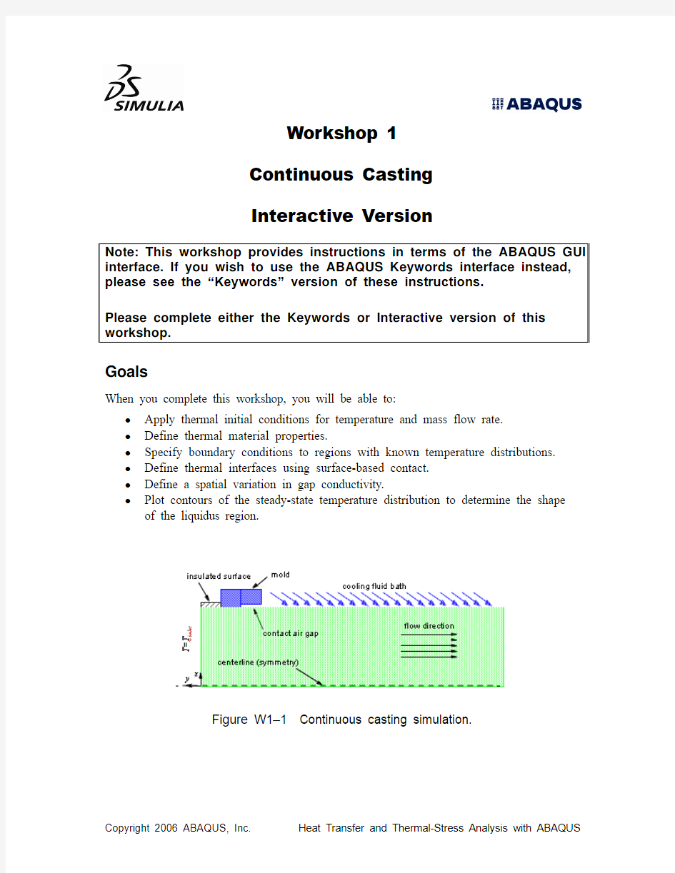
Figure W1–1 Continuous casting simulation.
W1.2
Introduction
In the continuous casting process shown in Figure W1–1, liquid aluminum (Al-0.7% Mg) is passed through a water-chilled mold to initiate the solidification process on the outer skin of the liquid. Water is then sprayed on the top and the bottom of the casting to continue the cooling process. The objective of this workshop is to determine the shape and the location of the freeze front under steady-state conditions.
Preliminaries
1. Enter the working directory for this workshop:
../heat_transfer/interactive/workshop1
2. Run the script ws_ht_casting.py using the following command:
abaqus cae startup=ws_ht_casting.py
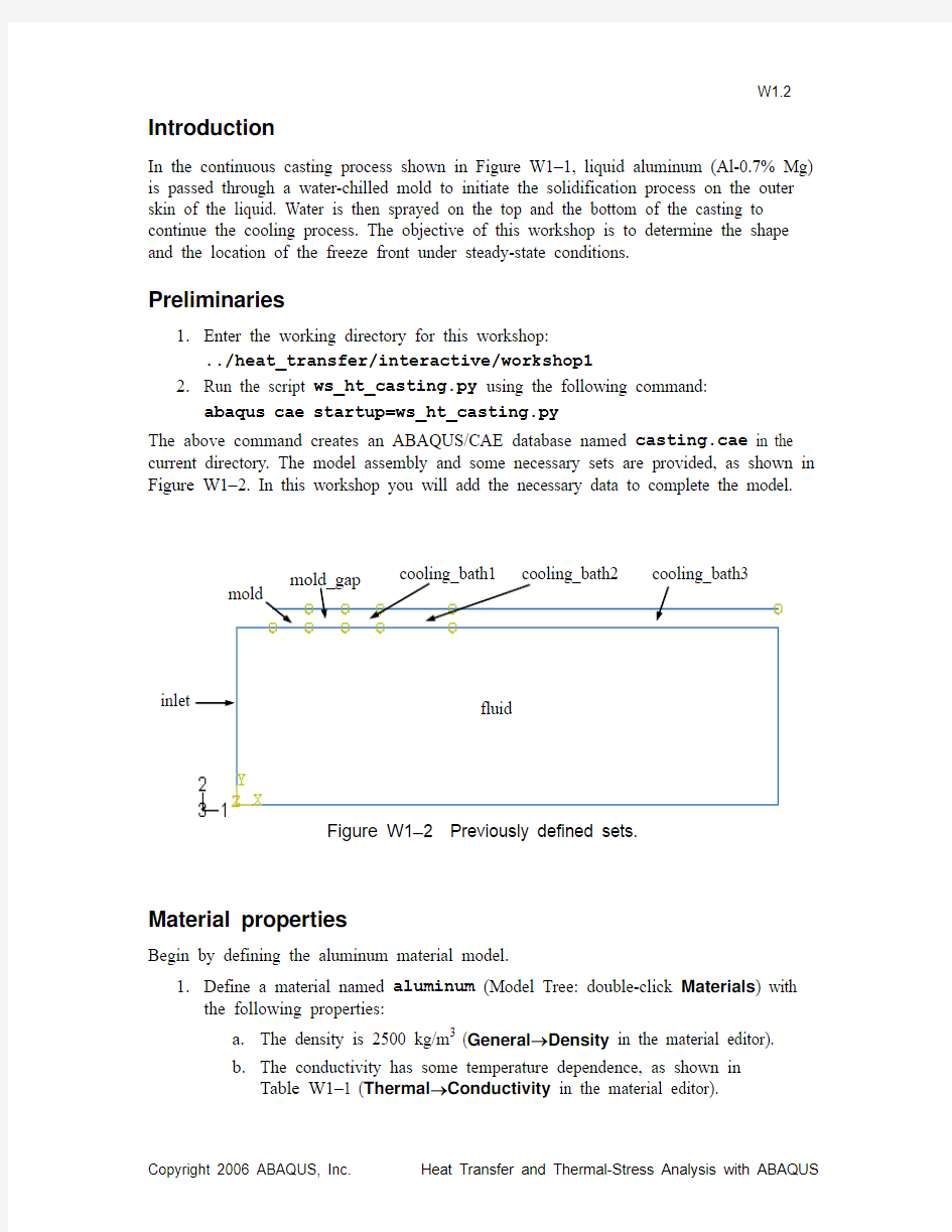
The above command creates an ABAQUS/CAE database named casting.cae in the current directory. The model assembly and some necessary sets are provided, as shown in Figure W1–2. In this workshop you will add the necessary data to complete the model.
Figure W1–2 Previously defined sets.
Material properties
Begin by defining the aluminum material model.
1. Define a material named aluminum (Model Tree: double-click Materials ) with the following properties:
a. The density is 2500 kg/m 3 (General →Density in the material editor).
b. The conductivity has some temperature dependence, as shown in
Table W1–1 (Thermal →Conductivity in the material editor). mold
mold_gap cooling_bath1 cooling_bath2 cooling_bath3
fluid
inlet
Table W1–1 Material conductivity.
Conductivity
W
m K
??
?
?
??
Temperature(K)
197.5 615
200.0 655
c.The specific heat of the aluminum is strongly temperature dependent; in
particular, the specific heat varies strongly with temperature between the solidus and liquidus temperatures to model the latent heat of solidification.
The variation of specific heat with temperature is shown in Table W1–2 (Thermal→Specific Heat in the material editor).
Table W1–2 Specific heat.
Specific heat
J
kg K
??
?
?
??
Temperature(K)
0.900 ? 103888
0.280 ? 106890
0.110 ? 107898
0.145 ? 107910
0.750 ? 106922
0.108 ? 104928
2.Create a homogeneous solid section named fluid using the material aluminum
(Model Tree: double-click Sections).
3.Assign the section fluid to the entire part fluid (Model Tree: Parts: fluid:
double-click Section Assignments).
Step definition
Next, you will define the steady-state heat transfer step and the step output requests.
1. Create a heat transfer step (Model Tree: double-click Steps ). Set the step
response type to steady state; ABAQUS automatically changes the default load
variation to ramp loads linearly over the step. Use a total step time of 1.0 and an
initial time increment of 0.001.
2. Modify the default field output request (Model Tree: Field Output Requests : double-click F-Output-1) to request variable HFLA , heat flux leaving the slave
surface, in addition to the default output variables: NT , nodal temperature; RFL ,
reaction flux; and HFL , heat flux per unit area. Save the results only at the last
increment of the step.
Thermal interfaces
The mold and bath are modeled as a series of line elements that share a thermal interface with the surface of the aluminum. The thermal interfaces between the aluminum and the mold and bath are modeled using contact with heat conductance through the gap. There are five separate thermal interface regions: the mold directly in contact with the
aluminum, the mold with an air gap, and the bath region (which is broken up into three parts). For each region there must be a surface on the aluminum casting and a node-based surface on the mold/bath side of the thermal interface. Each region also has its own values for gap conductance that have been determined experimentally.
1. Define the surfaces shown in Figure W1–3 on the free surface of the aluminum (Model Tree: Assembly : double-click Surfaces ).
Figure W1–3 Surfaces on the aluminum casting.
2. Define the interaction properties for the regions associated with the mold. Use the procedure provided below. The gap conductance for the part of the mold that
directly contacts the aluminum casting is 3000 W/m 2 K. The gap conductance for the region with an air gap between the mold and the aluminum casting is 100
W/m 2 K.
a. In the Model Tree, double-click Interaction Properties .
fluid_under_mold fluid_under_gap fluid_under_bath1 fluid_under_bath2 fluid_under_bath3
https://www.doczj.com/doc/e311076812.html, the contact property mold.
c.In the Edit Contact Property dialog box, select Thermal→Thermal
Conductance.
d.Modify the thermal conductivity table so that the conductivity will be
3000 for clearance values less than or equal to 1 (a large number
compared to the model dimensions) by entering the following
conductivity-clearance data pairs (3000, 0.0) and (3000, 1.0).
Tip: To insert a new row in the table after the first, click the third mouse
button while holding the cursor over the first row and select Add Row
After.
e.In order to complete the thermal conductivity table, a clearance value must
be specified at which the conductivity will be zero. Enter the following
data pair to satisfy this requirement: (0.0, 1000.0).
f.Click OK.
g.Repeat the above steps to define a property named gap with a
conductivity of 100 for clearance values of 1 or less.
3.The gap conductance in the bath varies with position, as determined previously by
experiment. The experimental data have been simplified. Three regions of the bath use different values for gap conductance, as shown in Table W1–3. Use the procedure provided in the previous step to define the interaction properties for the three bath regions. Name the interaction properties bath1, bath2, and bath3.
Table W1–3 Gap conductance for the regions of the bath.
Region Gap conductance
W
2
m K ?? ? ????
BATH1 1.7 ? 104
BATH2 1.3 ? 104
BATH3 1.1 ? 104
4.Define the contact interactions between the surfaces on the aluminum casting and
their corresponding node-based surfaces on the mold/bath. Each contact pair
definition must refer to the appropriate surface interaction.
a.In the Model Tree, double-click Interactions.
https://www.doczj.com/doc/e311076812.html, the surface-to-surface contact interaction mold.
c.When you are prompted to select the master contact surface, click
Surfaces in the prompt area. In the Region Selection dialog box, select
fluid_under_mold and click Continue.
W1.6
d.In the prompt area, choose Node Region as the slave surface typ
e. In the
Region Selection dialog box, select the set mold as the slave surface.
e.In the Edit Interaction dialog box, select mold as the interaction property
and click OK.
f.Repeat this procedure to define the following interactions:
?interaction gap between surface fluid_under_gap and node region mold_gap using interaction property gap,
?interaction bath1 between surface fluid_under_bath1 and node region cooling_bath1 using interaction property bath1,
?interaction bath2 between surface fluid_under_bath2 and node region cooling_bath2 using interaction property bath2, and ?interaction bath3 between surface fluid_under_bath3 and node region cooling_bath3 using interaction property bath3.
Initial conditions
The initial temperature and flow rate of the aluminum must be defined. The initial temperature in the aluminum is 1200K. The entire aluminum casting has a constant mass flow rate of 1.058?10-3 kg/s·m2 in the 1-direction (along the long axis of the casting).
1.Create a temperature field (Model Tree: double-click Fields) in the initial step
to assign an initial temperature of 1200 to the set fluid.
2.Currently, the mass flow rate cannot be defined directly through the
ABAQUS/CAE interface. However, you can use the keyword editor to define the initial aluminum flow rate using the procedure described below. This rate will
remain unchanged throughout the analysis.
a.In the Model Tree, click mouse button 3 on the model named casting and
select Edit Keywords in the menu that appears.
b.In the Edit keywords, Model: casting dialog box each keyword option is
displayed in its own option block. Select the *Initial conditions option
block and click Add After to add an empty text block.
c.In the new text block, enter the option shown below to define a mass flow
rate of 1.058e-3 through the set fluid:
*Initial conditions, type=mass flow rate
fluid, 1.058e-3, 0.0
d.Click OK.
Temperature boundary conditions
The upstream boundary condition consists of a fixed inlet temperature of 1200K, while the downstream condition allows convection but no axial conduction. Hence, no boundary conditions are required at the downstream edge.
W1.7
1.Define the upstream temperature boundary condition in Step-1 so that the set
inlet has a fixed temperature of 1200 (Model Tree: double-click BCs).
2.The part of the mold that is nearest the inlet is in direct contact with the aluminum.
The mold is kept at a constant low temperature to help cool the aluminum quickly.
The temperature varies with position in the mold from 300K to 304K. This
boundary condition is applied using the user subroutine DISP defined in the file
casting_udisp.f (or casting_udisp.for if you are working on a Windows system).
Create the mold temperature boundary condition in Step-1 so that the
temperature variation in the set mold will be applied using a user-defined
distribution with a magnitude of 1 (i.e., in the boundary condition editor, choose
User-defined in the Distribution field and enter 1 in the Magnitude field).
3.Next to the part of the mold that is in direct contact with the aluminum is a part of
the mold that has an air gap between the mold and the aluminum. This part of the
mold is kept at a constant temperature of 305K.
Apply a uniform temperature boundary condition of 305 to the set mold_gap.
4.Similar to the mold, the bath has a temperature distribution that varies with
position. The temperature in the bath ranges from 305K to 335K. As with the
mold, the temperature variation in the bath is applied using the user subroutine
DISP defined in the file casting_udisp.
Merge the sets cooling_bath1, cooling_bath2, and cooling_bath3 into a single set named bath (Model Tree: Assembly: [Control]+click the three sets,
click mouse button 3, and choose Merge in the menu that appears). Then apply a
temperature boundary condition to the merged set using a user-defined
distribution and a magnitude of 1.
Mesh
The aluminum is modeled with two-dimensional forced convection/diffusion (DCC2D4) heat transfer elements. The mold and bath are modeled with two-node heat transfer line elements (DC1D2). The mesh is already defined in the model. You can query the mesh attributes in the Mesh module (Tools Query).
Submit the analysis job
Recall, that the temperature boundary conditions defined for the mold and the bath require the user subroutine DISP defined in the file casting_udisp. The job for this analysis must refer to the user subroutine file.
1.Create a job named casting for the model casting (Model Tree: double-click
Jobs).
2.In the job editor, click the General tab and enter the user subroutine file name
(casting_udisp.f for UNIX or casting_udisp.for for Windows).
W1.8
3.Submit the job for analysis (Model Tree: Jobs: click mouse button 3 on casting:
Submit). Check the job monitor (Model Tree: Jobs: click mouse button 3 on
casting: Monitor) for any modeling errors and make any necessary corrections.
View the results
After the analysis has run to completion, study the analysis results.
1.In the Visualization module, open casting.odb.
https://www.doczj.com/doc/e311076812.html,e the Views toolbox (View→Views Toolbox) to apply the front view so that
the plot is oriented as shown in Figure W1–1.
3.Contour the steady-state temperature distribution.
a.From the main menu bar, select Result→Field Output.
b.In the Field Output dialog box, select NT11 (nodal temperature) as the
primary variable. Click OK.
c.In the Select Plot State dialog box, choose Contour and click OK.
4.Change the maximum contour limit to 900 and the minimum limit to 850 using
procedure provided below. In the resulting contour plot, the colored contour
region is in the temperature range of 850K to 900K, which is the liquidus
temperature for this alloy of aluminum.
a.In the toolbox, click the Contour Options tool .
b.In the Contour Plot Options dialog box, click the Limits tab. Enter 900
as the maximum contour limit and 850 as the minimum contour limit.
Click Apply.
c.When you have finished viewing the plot, click Defaults in the in the
Contour Plot Options dialog box to reset the contour limits to the default
values. Click OK.
5.Plot contours of heat flux leaving the slave surface (HFLA) for each contact pair.
a.From the main menu bar, select Result→Field Output.
b.In the Field Output dialog box, increase the width of the variable name
field until the surface names associated with the HFLA variables are visible.
(Adjust the column width by dragging the right edge of the Name column
title box.)
c.Select any of the HFLA variables and click Apply to plot contours of heat
flux leaving the slave surface. Repeat this step to plot HFLA for each
contact pair.
Note: A script that creates the complete model described in these instructions is available for your convenience. Run this script if you encounter difficulties following the instructions outlined here or if you wish to check your work. The script is named ws_ht_casting_answer.py and is available using the ABAQUS fetch utility.