INTERNATIONAL JOURNAL FOR NUMERICAL METHODS IN ENGINEERING
Int.J.Numer.Meth.Engng2008;76:314–336
Published online18March2008in Wiley InterScience(https://www.doczj.com/doc/3d92073.html,).DOI:10.1002/nme.2327
Ef?ciency of mixed hybrid?nite element and multipoint?ux
approximation methods on quadrangular grids and highly
anisotropic media
Anis Younes1,?,?and Vincent Fontaine2
1Institut de M′e canique des Fluides et des Solides,Universit′e Louis Pasteur de Strasbourg-CNRS/UMR7507
2rue Boussingault,F-67000Strasbourg,France
2Laboratoire de Physique des B?a timents et des Syst`e mes,Universit′e de la R′e union,15Avenue Ren′e Cassin,
BP7151-97715Saint-Denis Cedex09La R′e union,France
SUMMARY
The mixed hybrid?nite element(MHFE)and the multipoint?ux approximation(MPFA)methods are well suited for anisotropic heterogeneous domains since both are locally conservative and can handle general irregular grids.In this work,behaviours and performances of MHFE and MPFA methods are studied numerically for different heterogeneities and anisotropy factors on parallelograms and then on a more general quadrilateral grid.
The superiority of MPFA in terms of accuracy and ef?ciency is clearly demonstrated for parallelogram grids.In the case of more general quadrilateral grids,MPFA becomes more central processing unit time consuming than MHFE.For high anisotropy factors,both methods give results with signi?cant non-physical oscillations.Copyright2008John Wiley&Sons,Ltd.
Received8December2006;Revised6December2007;Accepted16January2008
KEY WORDS:mixed hybrid?nite element;multipoint?ux approximation;continuity point;high anisotropy;heterogeneous media;quadrilateral mesh
1.INTRODUCTION
We consider the numerical solution of the following partial differential equations(PDEs)on a2D quadrilateral grid:
?·q=f in (1a)
q=?K?P in (1b)
Correspondence to:Anis Younes,Institut de M′e canique des Fluides et des Solides,Universit′e Louis Pasteur de Strasbourg-CNRS/UMR75072rue Boussingault,F-67000Strasbourg,France.
?E-mail:younes@imfs.u-strasbg.fr
Copyright2008John Wiley&Sons,Ltd.
EFFICIENCY OF MHFE AND MPFA315 P=P e on* D(1c)
?K *P
*
=g on* N
where is a bounded polygonal open set of R2,* D and* N are partitions of the boundary* of corresponding to the Dirichlet(where P is?xed to P e)and the Neumann(where the?ux is ?xed to g)conditions,and the unit outward vector normal to the boundary* .
This set of equations,which leads to a diffusion-type PDE when(1b)is substituted in(1a),is a very common mathematical model in physics used to simulate diffusion processes such as heat or mass transfer or?ow in porous media.In the context of?ow in porous media,considered in this paper,the state variable P corresponds to the pressure or the piezometric head,q is the Dracy velocity,and K is a symmetric and positive de?nite permeability tensor.The components of K are assumed to be bounded but may be highly anisotropic and discontinuous.Indeed,full parameter tensors appear often for?ow in natural porous media when the grid orientation and geometry of the geological layer do not match.Moreover,for solute transport in porous media,the parameter tensor is a function of the?uid velocity and,therefore,for non-uniform?ow,has often signi?cant off-diagonal terms and is highly variable,whatever be the grid orientation.
Both the mixed hybrid?nite element(MHFE)and the multipoint?ux approximation(MPFA) methods are well suited for the discretization of(1c).Indeed,both are locally conservative and handle general irregular grids with anisotropic and heterogeneous permeability.
The mixed?nite element(MFE)method[1–4]approximates simultaneously the pressure P and the?ux q.The discretization of system(1c)leads to an inde?nite system matrix for the standard MFE method,which is circumvented by hybridization.The system is solved in this case for one unknown,the pressure Lagrange multipliers at element edges or faces.
In contrast to the MFE method,the MPFA method gives?uxes at cell interfaces explicitly by weighted sums of discrete node pressures.The MPFA discretization is a control volume formulation, where more than two pressure values are used in the?ux approximation.The?rst derivation of the methods was published in1994[5,6]and later in[7,8].The MPFA method can be applied in the physical space or in the reference space.Reference-space discretizations are symmetric,but their convergence diminishes or vanishes for rough grids[9].On the other hand,physical-space approximations have good convergence properties but are non-symmetric for quadrilaterals that are not parallelograms[9].The reason for the lack of symmetry was?rst presented in[10,11]. When numerical approximations or quadrature rules are used,relationships can be found between MPFA variants and MFE methods[12].The reference-space MPFA method was shown to be equivalent to the MFE method with a broken Raviart–Thomas space and speci?c quadrature rule in[13].However,the method requires asymptotic h2-parallelogram grids.An alternative analysis of essentially the same method,with the same grid restriction,is performed in[14,15]using a relation to the lowest-order Brezzi–Douglas–Marini element instead.
In[16],a MFE method with broken Raviart–Thomas elements and non-conventional quadrature rule is shown to be equivalent to the physical-space-derived MPFA method proposed by Aavatsmark et al.[17].
The MPFA and MFE methods lead to?nal systems with different properties(as,for example,the total number of unknowns,condition number,symmetry,stability,central processing unit(CPU) time requirement,number of non-zero values per row,etc.).In this work,we study the behaviour and the ef?ciency of both methods for high-anisotropic heterogeneous porous media.
Copyright2008John Wiley&Sons,Ltd.Int.J.Numer.Meth.Engng2008;76:314–336
316
A.YOUNES AND V .FONTAINE
2.THE MFE METHOD
The MFE method uses both the velocity and the pressure as primary unknowns simultaneously.MFE has many well-known estimates on the variables [1–3].This includes superconvergence for both the velocity and the pressure in the case of smooth permeability and a suf?ciently smooth grid [18].
The discretization of (1c)leads to an inde?nite system matrix for the standard MFE method,which is circumvented by hybridization.The system is solved in this case for the pressure on the edges,viewed as the Lagrange multipliers.This form of the MFE method is called MHFE method.A relationship between the MFE method and cell-centred ?nite differences,via low-order numerical integration,was pointed out by Russell and Wheeler [19]for K -orthogonal grids.These results were extended to full tensor coef?cient by Arbogast et al.[20,21]by introducing the expanded MFE method,which adds the pressure-gradient variable as one of the primary unknowns.However,this method loses accuracy near discontinuities and pressure Lagrange multipliers have to be introduced along discontinuous interfaces to recover higher-order convergence.
A ?nite volume formulation of the MHFE method was obtained without any numerical quadra-ture rule for triangular meshes in [22–24].
For the test problem (1c)with heterogeneous anisotropic domain and general quadrilateral geometry,the MHFE method remains the best-suited variant of the MFE method.2.1.The MHFE formulation
The Raviart–Thomas space over quadrilateral elements is de?ned with the help of a reference
square element E
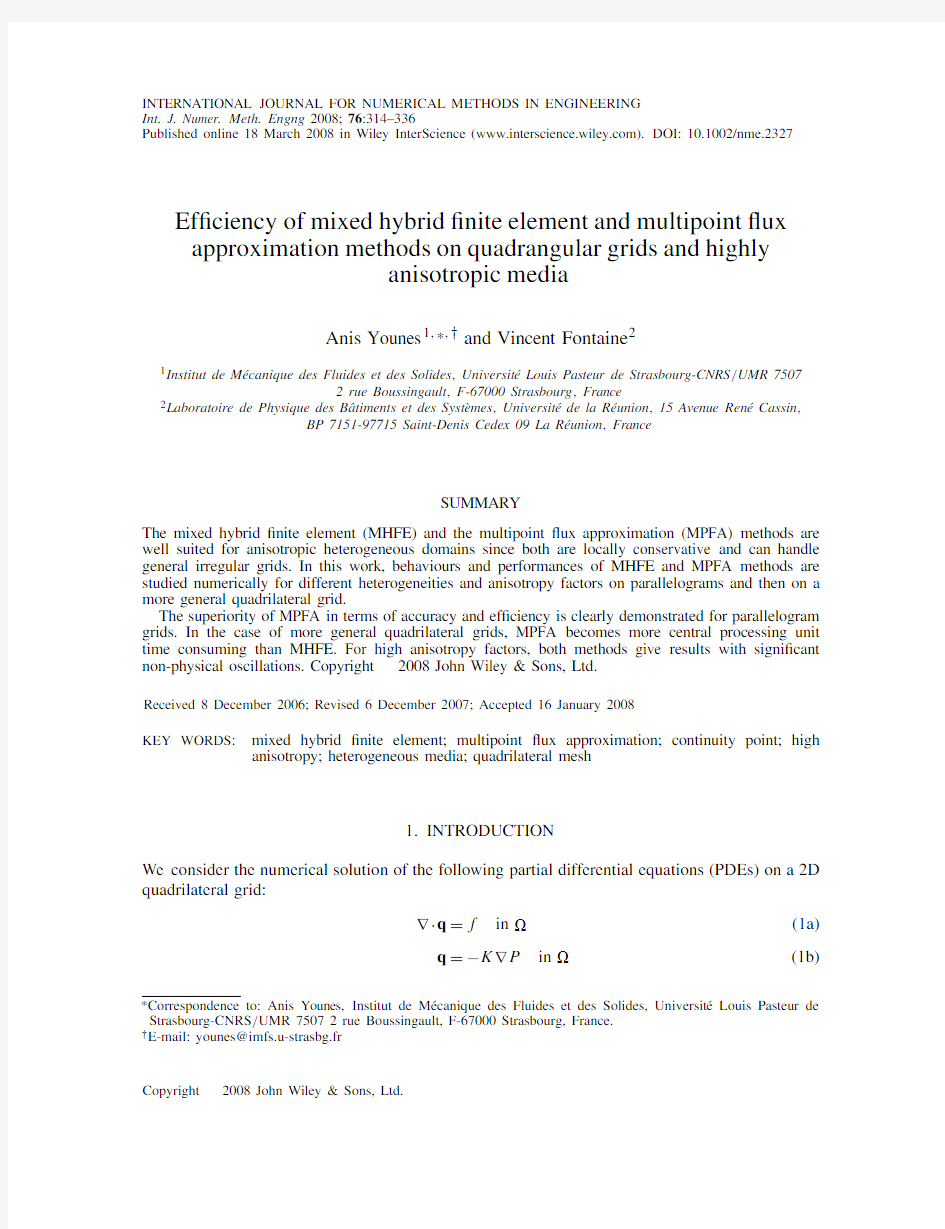
.For any cell E ,we utilize a bilinear mapping F =F E : E
→E (see Figure 1).Let J be the Jacobian matrix and |J |its determinant.Let x i =(x i ,y i ),i =1,2,3,4,be the four vertices of element E in a counterclockwise direction and x i j =x i ?x j .If x 1=(0,0)T , x 2=(1,0)T , x 3=(1,1)T ,and x 4=(0,1)T ,then
F E (
x , y ):x 1+x 21 x +x 41 y +(x 32?x 41) x y We consider the quadrilateral element E with four edges E i .The solution (P ,q )to Equation (1c)is approximated over E ,by the following quantities:
?P E ∈R :the mean value of P over the element E ;
?TP E i ∈R :the mean value of P over the edge E i ,i =1,...,4;?q E ∈X E :the approximation of q =?K ?P over E .
1
x 2
x
2
3
x Figure 1.Bilinear mapping from the reference to the physical element.
Copyright 2008John Wiley &Sons,Ltd.
Int.J.Numer.Meth.Engng 2008;76:314–336
EFFICIENCY OF MHFE AND MPFA
317
where X E is the lowest-order Raviart–Thomas space [1,2]and q E can be expressed as
q E =
4 i =1
Q E i x i
(2)
where Q E i denotes the ?ux leaving E through the edge E i ,which is taken positive outwards.
The basis function x i veri?es [1,2]
E j
x i · E j = i j (3)
which leads to
E
?·x i =1(4)
A basis of X E in the square reference element E
=[0,1]×[0,1]is given by x 1= x 0 , x 2= x ?10 , x 3= 0 y , x 4=
0 y ?1
(5)
Using properties (3)and (4),the modi?ed Darcy’s law (K ?1q =??P )expressed in a variational
form leads to
E
K ?1q E x i =4 j =1
Q E j
E
x i K ?1x j =? E
?P x i =
E
P ?·x i ?
E j
P x i · E j =P E ?TP E
i (6)
We now introduce local matrix notations on element E :
B =[B i j ]with B i j =
E
x i ·K ?1·x j
(7)
B i j is evaluated in the reference space using
B i j =
E
x i · K ?1· x j (8)
where K
?1=J T K ?1J /|J |corresponds to the analogue tensor in the reference element.The Jacobian matrix is constant only when the grid cells are parallelograms.B i j is generally evaluated with numerical integration using Gaussian points or the corners of the grid.The matrix B is symmetric and positive de?nite.Equation (6)can be expressed as
Q E i =
4 j =1
B ?1i j (P E ?TP E j )
(9)
The mass balance equation (1a)is discretized using a ?nite volume formulation in space:
E
?·q = E
?· 4 i =1
Q E
i x i = E
f
(10)
Copyright 2008John Wiley &Sons,Ltd.
Int.J.Numer.Meth.Engng 2008;76:314–336
318
A.YOUNES AND V .FONTAINE
Using (4)leads to
4 j =1
Q E j =|E |f E =Q E s
(11)
where f E is the mean value of f over the element E .
Combining (9)and (11),we obtain
P E
=4 i =1 i TP E
i +
Q E s (12)
with i = 4j =1B ?1
i j and = 4i =1 i .Replacing (12)in (9)leads to
Q E i =
i 4
j =1 j TP E j ?4 j =1
B ?1i j TP E j + i Q A s (13)
With the MHFE method,the scalar unknowns are TP E i ,i =1,...,n f for all elements E .The ?nal
system of equations is obtained using continuity properties as follows:
?On all interior edges,if i is the common edge of the two elements A and B ,then
TP A i =TP B
i and
Q A i +Q B i =0
(14)
?if i is a Dirichlet boundary edge,then
TP A i =TP bc
i
(15)
?if i is a Neumann boundary edge,then
Q A i =Q bc
i
(16)
where TP bc i and Q bc i
are the given values of P and Q at the Dirichlet and Neumann boundaries,respectively.
3.THE MPFA METHOD
The MPFA method has been developed as a ?nite volume method.It is accurate for rough grids and coef?cients and reduces to a cell-centred stencil for the pressures.
The basic idea is to divide each cell into subcells (Figure 2(a)).Inside the subcell of the corner
x i ,we assume linear variation of the pressure between the corresponding mid-point edges x 1i
and x 2i
and the centre of the element x (Figure 2(b)).Therefore,subedge (half-edge)?uxes,taken positive for out?ow,are given by
Q 1i Q 2i =1
2|T xx 1i x 2i
| (x 1i ?x i )⊥K (x 2i ?x )⊥(x 1i ?x i )⊥K (x ?x 1i )⊥(x i ?x 2i )⊥K (x 2i ?x )⊥(x i ?x 2i )⊥K (x ?x 1i )⊥ G E
i 1i ?P E 2i
?P E (17)Copyright 2008John Wiley &Sons,Ltd.
Int.J.Numer.Meth.Engng 2008;76:314–336
EFFICIENCY OF MHFE AND MPFA
319
2
3
x
x 1
i Q 2
i Q (a) (b)
Figure 2.Cell splitting into four subcells and linear pressure approximation on each subcell.
Figure 3.The interaction region sharing the vertex i .
where |T xx 1i x 2i
|is equal to the area of the triangle spanned by the points x ,x 1i ,and x 2i ;for example,the vector (x 1i ?x i )⊥is obtained by a rotation of the vector x 1i
?x i with an angle of /2.All subcells sharing the vertex i create an interaction volume (see Figure 3).
The discretization is accomplished by assuming continuous ?uxes across each of the subedges and a weak continuity condition of the pressure across the same edges.From these assumptions,an explicit discrete ?ux can be found after resolution of a local linear system and eliminating the edge pressure for each subedge of the interaction volume (details are given below for the simpler rectangular case).Each subedge ?ux can then be expressed explicitly as a weighted sum of the cell pressures of the interaction volume.For example,for Figure 3we obtain
Q 1i =
4 k =1
t k i P E k
(18)
where t k i are transmissibility coef?cients (developments are given in the following section for
rectangular meshes).
3.1.Symmetric or non-symmetric MPFA method
The ?nal system is obtained when the mass balance is expressed for each cell:sum of all subedge ?uxes of the cell equals the sink /source term over that cell.Unfortunately,the resulting mass matrix is generally non-symmetric,which,for instance,slows down the computations.
Indeed,as shown in [17],symmetry of the global matrix is guaranteed only if this property is
respected for each local matrix G E i .The symmetry is achieved when we replace in (17)(x 1i
?x )⊥and (x 2i ?x )⊥by (x i ?x 1i )⊥and (x i ?x 2i )⊥,respectively.The matrix G E i
is then approximated by Copyright 2008John Wiley &Sons,Ltd.
Int.J.Numer.Meth.Engng 2008;76:314–336
320
A.YOUNES AND V .FONTAINE
the following equation:
G
E i =1
2|T x 1i ,x i x 2i
|
(x 1i ?x i )K (x i ?x 2i )⊥
(x 1i ?x i )K (x i ?x 1i )⊥
(x i ?x 2i )K (x i ?x 2i )⊥
(x i ?x 2i )K (x i ?x 1i )
⊥
(19)
In the case of parallelograms,we have (x 1i ?x )⊥=(x i ?x 1i )⊥,(x 2i ?x )⊥=(x i ?x 2i
)⊥and then G E i = G E i .For general quadrilateral element,with G E i ,we approximate the quadrangular subcell x i ,x 2i ,x ,and x 1i
by the parallelogram x i ,x 2i , x ,and x 1i ,where the cell centre of the parallelogram has now moved away from the cell centre of the original quadrilateral (Figure 4).
The symmetric MPFA method uses G E i in place of G E i
for quadrilateral grids.In the case of rough grids,G E i and G E i can be very different contrarily to h 2-perturbed parallelograms where G E i
can be very close to G E i .The symmetric MPFA method was shown to be equivalent to two MFE
formulations,broken Raviart–Thomas [9,13,25]and Brezzi–Douglas–Marini [9,14,15]elements with a speci?c quadrature rule.Indeed,with both MFE formulations,a trapezoidal-type quadrature rule reduces the velocity mass matrix to a block diagonal form and leads to the same symmetric and positive de?nite cell-centred pressure system as with the symmetric MPFA discretization de?ned above.The relationship between MPFA and MFE was ?rst addressed in [12]and the symmetric MPFA formulation was ?rst presented in [10–12].
Convergence of both symmetric and non-symmetric MPFA methods was studied by many authors [9,13–16].For quadrilateral elements that are h 2-perturbation of parallelograms,the pressure and the normal velocity were shown to be second-order convergent for both symmetric and non-symmetric MPFA formulations.
For rough grids,i.e.grids with h -perturbation,the pressure still converges with rate O (h 2)for the non-symmetric MPFA discretization,whereas the convergence diminishes or vanishes for the symmetric one.Concerning the normal velocities,the rate of the convergence with the non-symmetric MPFA method decreases to O (h ),whereas the symmetric MPFA method suffers a loss of convergence [9].
3.2.Localization of continuity points
Continuity of the normal ?ux and pressure is generally prescribed at the element-edge mid-point.This corresponds to w =1(see Figure 5).However,as shown in [26],there is ?exibility in location
2
x 1
i Q 2
i Q Figure 4.Virtual cell-centre ?x
to obtain symmetric MPFA method.Copyright 2008John Wiley &Sons,Ltd.
Int.J.Numer.Meth.Engng 2008;76:314–336
EFFICIENCY OF MHFE AND MPFA321
2
3
2
3 2
3
(a)(b)
(c)
Figure5.Different locations of the pressure and velocity continuity point at the subcell interface.Local pressure support for w=1.0(a),w=0.5(b),and w=0.1(c).
of the continuity point.Its position can be chosen to lie at any point between the edge mid-point and the vertex(see Figure5(b)and(c)).
For parallelograms,the best choice is w=1,since it leads to a9-points,cell-centred?nite difference scheme with a symmetric positive de?nite matrix for general K tensor.Moreover,for K-orthogonal grids,it reduces to a5-points?nite difference scheme as will be shown in detail in the following section.
For rough grids,all continuity positions lead to non-symmetric matrices.Recent numerical results in[26]show that the location w=0.1improves convergence for discontinuous coef?cient problems with isotropic or mildly anisotropic coef?cients.The behaviour of the MPFA method with different w’s(different locations of the continuity point)and different anisotropy factors will be studied in Section5.
4.THE CASE OF PARALLELOGRAMS
In this section,we study the properties and numerical ef?ciencies of both MPFA and MHFE methods for parallelograms.In this case,the Jacobian is constant.For the MPFA method,the best choice for the location of the continuity point is the edge mid-point.In this case,G E i= G E i and the MPFA method is symmetric.
4.1.M-matrix property for rectangular grids
The M-matrix property(non-singular matrix with m ii>0and m i j 0)guarantees the respect of the discrete maximum principle,i.e.local maxima or minima will not appear in the P solution in a domain without local sources or sinks.This property ensures that the resulting numerical state variable P and its related?uxes q are consistent with the physics.
Let us consider the simple case of diagonal permeability tensor on a rectangular-shaped element x× y.
Copyright2008John Wiley&Sons,Ltd.Int.J.Numer.Meth.Engng2008;76:314–336
322 A.YOUNES AND V.FONTAINE
4.1.1.The MHFE method.For rectangular elements with diagonal permeability tensor,the system matrix with MHFE method is obtained when the continuity of?uxes(14)between two adjacent elements A and B is expressed.
From(13),the diagonal and off-diagonal terms of the?nal matrix are
m ii=
B?1ii?
2i
A
+
B?1ii?
2i
B
m i j=
B?1i j?
i j
A
(20)
The elemental matrix B?1is
B?1A=2?
??
??
??
2 A x A x00
A x2 A x00
002 A y A y
00 A y2 A y
?
??
??
??(21)
with
A x= y
K A x, A y=
x
K A y, 1= 2=6 A x, 3= 4=6 A y and =12( A x+ A y)
The diagonal term with MHFE is always positive,since
B?1ii> 2i/ for i=1,2,3,4(22) The off-diagonal term is negative if m i j 0for(i=j)which yields to the following conditions:
m12=B?112? 1 2
=
A x A y
x+ y
(2? A x/ A y) 0if A x/ A y 2(23)
m34=B?134? 3 4
=
A y A x
( x+ y)
(2? A y/ A x) 0if A x/ A y 1
2
(24)
Conditions(23)and(24)cannot be ful?lled at the same time.Therefore,the matrix system of MHFE is never an M-matrix in this case.
4.1.2.The MPFA method.In the case of rectangular elements with diagonal K,the local matrix
G E i is a diagonal matrix.The interaction region is a rectangle.If we use notations of Figure6, when continuity of?uxes and pressure across edges is expressed,we obtain the following linear Copyright2008John Wiley&Sons,Ltd.Int.J.Numer.Meth.Engng2008;76:314–336
EFFICIENCY OF MHFE AND MPFA323
Figure6.The interaction region in the case of a rectangular mesh.
system:
???
???????? (K B x+K A x)000
1
(K B y+K C y)00
00 (K C x+K D x)0
000
1
(K A y+K D y)
?
??
??
??
??
??
?
??
??
?
AB
BC
C D
AD
?
??
??
?
=
?
??
??
??
??
??
K A x K B x00
1
K B y
1
K C y0
00 K C x K D x
1
K A y00
1
K D y
?
??
??
??
??
??
?
??
??
?
P A
P B
P C
P D
?
??
??
?
(25)
where = y/ x.
The previous system is solved to obtain the pressure at edges AB, BC, C D,and AD and then subedge?uxes from(17):
Q AB= K A x K B x
x x
(P A?P B),Q BC=1
K B y K C y
y y
(P B?P C)
Q C D=
K C x K D x
(K C x+K D x)
(P C?P D),Q D A=1
K A y K D y
(K A y+K D y)
(P D?P A)
(26)
For the subedge?ux Q AB,the transmissibility coef?cient in(18)corresponds to t AB= K A x K B x/(K B x+K A x).
Copyright2008John Wiley&Sons,Ltd.Int.J.Numer.Meth.Engng2008;76:314–336
324 A.YOUNES AND V.FONTAINE
Hence,the mass balance equation over an element A(sum of the eight subedge?uxes equal to the sink/source term over A)leads to a5-points,cell-centred?nite difference scheme with a harmonic mean of permeabilities at interfaces.It is easy to see that the corresponding matrix is an M-matrix.
Remark
In the case of non-rectangular parallelograms with diagonal K or in the case of rectangular elements with a full permeability tensor,the left matrix in(25)becomes less sparse and the same analysis shows that the MPFA method leads to a9-points,cell-centred?nite difference scheme with a generalization of the harmonic mean of permeabilities.The obtained matrix is not,in general,an M-matrix[8].
The number of unknowns corresponds to the number of edges for the MHFE method and to the number of elements for the MPFA method.For an N x×N y rectangular grid,the MHFE method requires(2N x N y+N x+N y)unknowns,whereas the MPFA method has only N x N y unknowns. The properties of MPFA and MHFE methods in the case of parallelograms are given in Table I.
4.2.Numerical experiments
We de?ne the following test problem:system(1c)is solved on a unit square shape =(0,1)2 domain with anisotropic and heterogeneous permeability?eld.The tensor coef?cient and the true solution for the test problem are
K=
y2+ x2( ?1)xy
( ?1)xy x2+ y2
(27)
P(x,y)=exp(?20 ((x?1
2)2+(y?1
2
)2))(28)
In this paper,behaviours and properties of both methods are studied numerically for different anisotropy factors for two rectangular discretizations(30×30and100×100).Tables II and III give the coef?cient of anisotropy ( =1corresponds to the isotropic case),the total number of unknowns N unk,the number of iterations N it,and the CPU time t CPU obtained with the iterative preconditioned conjugate gradient(PCG)solver.The Eisenstat trick[27]is applied to the precondioned matrix and allows saving a signi?cant part of computation.Tables II and III
also give the CPU time t UMF
CPU obtained with UMFPACK4.4.It is a direct solver based on both
unifrontal/multifrontal methods adapted for solving sparse linear systems[28].This solver is in the public domain and can be implemented on a single processor workstation.Moreover, UMFPACK4.4.also gives a rough estimate of the reciprocal condition number Rcond(Tables II and III).
Table I.Matrix properties of MPFA and MHFE methods on parallelogram meshes.
M-matrix for M-matrix for Nb of non-zero Symmetric/rectangular mesh and rectangular mesh Nb of values per row positive de?nite diagonal K and full K unknowns for full K MHFE Yes No No Nb of edges7 MPFA Yes Yes No Nb of elements9 Copyright2008John Wiley&Sons,Ltd.Int.J.Numer.Meth.Engng2008;76:314–336
EFFICIENCY OF MHFE AND MPFA325 Table II.Matrix properties,CPU time consumption,and solution behaviours of MHFE and MPFA
methods on a30×30rectangular grid.
=1 =10 =100 =1000
Q Min,Max
s?0.0240.14?0.33210.7901?3.4617.288?34.7572.27
MPFA MHFE MPFA MPFA Methods MHFE w=1MHFE w=1MHFE w=1MHFE w=1 N unk1860900186090018609001860900
N it695077641428340494
t CPU6.2e?24.6e?26.2e?24.6e?27.2e?24.6e?20.14.6e?2 Rcond2.15e?12.94e?11.9e?12.1e?13.98e?29.16e?25.83e?35.14e?2 t UMF
9.3e?29.3e?29.3e?29.3e?29.3e?29.3e?29.3e?29.3e?2 CPU
P Min?2.7e?4?7.4e?4?1.2e?3?1.6e?3?0.144?2.0e?3?2.37?3.9e?3 P Max0.940.970.9760.97 1.410.98 5.810.98 ep L23.2e?38.9e?42.2e?32.3e?35.6e?22.8e?30.613.1e?3 ev L25.7e?33.4e?39.7e?29.7e?2 1.27 1.0113.510.18
Table III.Matrix properties,CPU time consumption,and solution behaviours of MHFE and MPFA
methods on a100×100rectangular grid.
=1 =10 =100 =1000
Q Min,Max
s?0.00220.0129?0.0310.0729?0.31990.6728?3.21 6.672
MPFA MPFA MPFA MPFA Methods MHFE w=1MHFE w=1MHFE w=1MHFE w=1 N unk2020010000202001000020200100002020010000 N it214160232198368258638286
t CPU0.920.750.950.797 1.230.86 1.730.9 Rcond1.6e?11.94e?11.45e?11.44e?13.02e?25.6e?24.09e?32.6e?2 t UMF
1.040.9 1.030.9 1.050.89 1.060.89 CPU
P Min?1.0e?5?4.7e?5?9.e?5?1.2e?4?1.2e?2?1.7e?4?0.183?4.3e?4 P Max0.9940.9970.9980.998 1.040.998 1.470.998 ep L22.9e?47.9e?52e?42.11e?45.3e?32.5e?45.8e?22.8e?4 ev L25.4e?43.1e?48.9e?38.8e?30.1229.2e?2 1.360.92
The condition number of a matrix is the product of its norm and the norm of its inverse.It can be viewed as a measure of how close a matrix is to a rank-de?cient matrix.It can also be viewed as a factor by which errors in solving linear systems with this matrix as a coef?cient matrix could be magni?ed.Condition numbers are usually estimated,since exact computation is costly in terms of?oating-point operations.Matrices are well conditioned if the reciprocal condition number is near1and ill-conditioned if it is near zero.
The sink source term of the test problem is calculated for each element in order to obtain the desired solution.Its continuous expression is obtained by substituting(27)–(28)into system (1a)–(1b).It corresponds to an injection at the centre of the domain located between two sinks
Copyright2008John Wiley&Sons,Ltd.Int.J.Numer.Meth.Engng2008;76:314–336
326 A.YOUNES AND V.FONTAINE
(Figure7).The magnitude of sink/source terms increases when anisotropy increases(Tables II and III).
Pressure errors and normal velocity errors are investigated in the discrete L2-norms,which are de?ned as in[29]by the expressions:
ep L2=
i
(|A i|(P an,i?P i))1/2(29)
ev L2=
j
|E e,j|((Q an,j?Q j)|e j|)2
j
|E e,j|
1/2
(30)
Here|A i|is the area of grid cell i,|E e,j|is the area associated with cell edge j(equal to half the sum of the areas of two neighbouring grid cells),and cell edge j has length equal to|e j|.The analytical pressure P an,i is evaluated at the node of cell i,whereas the analytical?ux Q an,j of cell edge j is evaluated by the mid-point rule.
Results of numerical experiments for rectangular meshes(Tables II and III)show the following:?For the same problem,the MPFA method requires50%less unknowns than the MHFE method.
?The number of iterations for the iterative solver,and therefore the total CPU time,increases when the anisotropy factor increases.
Figure7.The distribution of the sink/source term for the anisotropy =100.
Copyright2008John Wiley&Sons,Ltd.Int.J.Numer.Meth.Engng2008;76:314–336
EFFICIENCY OF MHFE AND MPFA327?The CPU time with the direct solver remains constant even when increases.
?The MPFA matrix is in general better conditioned than the MHFE matrix.This phenomenon is more pronounced for high .Indeed,for =1000,the reciprocal condition number is10 times greater with MPFA than with MHFE for the coarse discretization.
?MPFA is less time consuming than MHFE,especially for high .Indeed,with the iterative solver,the MPFA method requires25%less CPU time than MHFE for =1and50%less CPU time for =1000.
?The numerical solution for the pressure should be between0and1.The MHFE method gives a solution with signi?cant oscillations(a minimum pressure value P min=?2.37and a maximum value P max=5.81)on the coarse grid(Figure8).These oscillations are reduced with the?ne grid(P min=?0.183and P max=1.47).
?The non-physical oscillations are avoided or strongly reduced with the MPFA method (Figure9).Indeed,the pressure solution has a minimum P min=?3.9e?3and a maximum P max=0.98for =1000on the coarse mesh.These oscillations are reduced for the?ne discretizations(P min=?4.3e?4and P max=0.998).
?The pressure error with MPFA is much smaller than with MHFE especially for high .Indeed, for =1000,the pressure error is200times less important with MPFA than with MHFE.?The velocity error is also reduced with the MPFA method.For =1000,MPFA gives50% less velocity error than MHFE.
Figure8.The MHFE pressure solution for =1000on the coarse grid.
Copyright2008John Wiley&Sons,Ltd.Int.J.Numer.Meth.Engng2008;76:314–336
328
A.YOUNES AND V .FONTAINE
Figure 9.The MPFA pressure solution for =1000on the coarse grid.
?The pressure and velocity errors are given for different meshes for =300in Figure 10.These errors are smaller with MPFA than with MHFE and retain the same behaviour for both methods when the mesh is re?ned.
MPFA and MHFE methods are well suited for problems with discontinuous coef?cients.To show the velocity error in this case,we simulate the following test problem with the non-diagonal discontinuous K :
K =????????? 10225 ,x <1/2
1001 ,x >1/2
(31)The exact solution is
P (x ,y )=??????????? 1+ x ?12 110+8 y ?12 exp ?20 y ?12
2
,x <1/2
exp x ?12 exp ?20 y ?12
2 ,x >1/2(32)
Copyright 2008John Wiley &Sons,Ltd.
Int.J.Numer.Meth.Engng 2008;76:314–336
EFFICIENCY OF MHFE AND MPFA329
Figure10.Pressure and velocity errors with MHFE and MPFA S for different rectangular meshes.
Figure11.Pressure and velocity errors with MHFE and MPFA S for different rectangular
meshes for discontinuous coef?cients.
As for the continuous case,MPFA gives smaller velocity error than MHFE.When the mesh is re?ned the same behaviour is observed with both methods(Figure11).
These numerical results show that when applied on parallelograms,the MPFA method has less unknowns and is more ef?cient and more accurate than the MHFE method,especially for high anisotropic media.These results can reasonably be generalized to asymptotic h2-parallelogram grids since the symmetric MPFA formulation has the same performance and behaviour as with parallelograms[13–15].
5.THE CASE OF GENERAL QUADRILATERAL GRID
In this section,behaviour and numerical ef?ciency of both MPFA and MFE methods for general unstructured quadrilateral grids are studied.For rough grids,G E i and G E i can be very different and the MPFA method leads to a non-symmetric matrix.Approximating G E i by G E i,in order to Copyright2008John Wiley&Sons,Ltd.Int.J.Numer.Meth.Engng2008;76:314–336
330 A.YOUNES AND V.FONTAINE
obtain a symmetric MPFA formulation,induces large errors since geometry of the cell is only approximately honoured.In this case,a loss of convergence can be observed for the symmetric MPFA formulation[9].
When using the standard MPFA formulation on general quadrilateral grid,the localization of the continuity point can be different from the edge mid-point since the obtained matrix is always non-symmetric for whatever be the localization of the continuity point between the edge mid-point and the vertex.The behaviour of the MPFA method with different w(different localizations of the continuity point)for different anisotropy factors is studied in this section.
The use of the general quadrilateral grid with both MHFE and MPFA methods is more compli-cated than parallelograms.Indeed,with the MHFE method,the Jacobian matrix is no more constant. The elements B i j of the local matrix in(8)cannot be evaluated exactly and we resort to numerical integration.Accuracy and performance of MHFE with Gaussian quadrature(we use seven inte-gration points at Gaussian locations)and with corner quadrature(we use four integration points at the corners of the grid)will be tested.
Moreover,for general quadrilateral grids,the interaction volume of the MPFA method can include more than four elements.This will make the larger non-symmetric local system to inverse for each node of the grid,which can be time consuming.As a consequence,the?nal non-symmetric matrix system can be less sparse than the MHFE one,since the number nbv of neighbours sharing the considered cell can be important.
The properties of MPFA and MHFE methods for a general quadrilateral grid are summarized in Table IV.Contrary to the case of parallelograms,it is not obvious from Table IV that the MPFA method will be competitive with the MHFE method in this case.
Again,the iterative solver with MHFE method is the PCG solver since the matrix is always symmetric and positive de?nite.However,with the MPFA method,we use the bi-conjugate gradient stabilized iterative solver since the obtained matrix is non-symmetric.The residual for both solvers is10?16and the maximal number of iterations is105.
5.1.Numerical experiments
A general quadrilateral grid is obtained from the previous30×30rectangular grid.Each rectangle of the previous regular mesh is subdivided into?ve quadrilaterals as shown in Figure12.The obtained quadrangular mesh is plotted in Figure13.Note that nodes of this mesh can have eight surrounding elements.In this case,the interaction volume of MPFA includes eight elements and leads to the inversion of a local(8×8)non-symmetric system.Note also that cells in Figure13 can have14neighbours sharing the considered cell,which leads to15non-zero values per row in the?nal non-symmetric matrix of MPFA.
The results of MHFE and MPFA methods for the test problem(27)on the rough grid of Figure13 are given in Tables V and VI for different anisotropy factors(1 103).The results of MHFE Table IV.Matrix properties of MPFA and MHFE methods for general quadrilateral grids.
Symmetric/positive M-matrix for general Number of Number of non-zero de?nite quadrilaterals unknowns values per row MHFE Yes No Nb of edges7
MPFA No No Nb of elements nbv 9 Copyright2008John Wiley&Sons,Ltd.Int.J.Numer.Meth.Engng2008;76:314–336
EFFICIENCY OF MHFE AND MPFA
331
00,0
x,y
0,y
Figure 12.Splitting of a
rectangle into ?ve irregular quadrangles.
Figure 13.The general quadrilateral discretization obtained from the 30×30rectangular mesh.
are given for both Gaussian and corner quadratures and the MPFA results are given for different w (different localizations of the continuity point).
The results of numerical experiments (Tables V and VI)show the following:
?MHFE with Gaussian quadrature is better conditioned than with corner quadrature.Both formulations require similar CPU time.However,non-physical oscillations are more signi?-cant with the corner quadrature rule.
?MHFE with Gaussian and corner quadratures leads to similar pressure and velocity errors in the case of isotropic medium ( =1).When increases,the Gaussian quadrature leads to smaller errors than the corner quadrature.
Copyright 2008John Wiley &Sons,Ltd.
Int.J.Numer.Meth.Engng 2008;76:314–336
332
A.YOUNES AND V .FONTAINE
T a b l e V .C o m p a r i s o n s o f m a t r i x p r o p e r t i e s ,C P U t i m e c o n s u m p t i o n ,a n d s o l u t i o n b e h a v i o u r s o f m i x e d a n d M P F A m e t h o d s o n a q u a d r a n g u l a r 30×30g r i d u s i n g a l a r g e r a n g e o f a n i s o t r o p y v a l u e ,1 102.
=1 =10 =100
M H F E
M P F A
M H F E
M P F A M H F E
M P F A
M e t h o d s
G a u s s C o r n e r
w =0.1w =0.5w =0.9w =1.0
G a u s s C o r n e r
w =0.1w =0.5w =0.9
w =1.0
G a u s s
C o r n e r w =0.1w =0.5
w =0.9w =1.0
N u n k 906045009060
450090604500
N i t 29825998106119125286287167
145168X 446464X X X X
t C P U (s )0.430.420.370.390.420.430.450.430.50.470.51X 0.580.58X X X X R c o n d 9.5e ?28e ?22.7e ?12.4e ?21.6e ?11.4e ?16.1e ?26.3e ?28.9e ?31.3e ?19.2e ?27.6e ?52e ?21.4e ?21.9e ?59.9e ?67.6e ?72.8e ?7t U M F C P U
(s )0.430.420.470.470.460.460.420.420.480.460.480.480.420.420.480.470.480.48P M i n ?2.7e ?2?1.3e ?2?3e ?4
?1.6e ?4
?2.8e ?5
?7.5e ?5?5.9e ?4?6.2e ?4
?6.2e ?4
?6.3e ?4
?.35e ?4
?2.4e ?4?0.149?0.29
?0.13?9e ?3?3.1e ?3?287
P M a x
0.980.990.9880.9860.9860.9851.021.050.9880.9860.980.981.531.821.0130.990.97129.3e p L 21.2e ?31.3e ?3
1.3e ?3
1.0e ?3
6.9e ?4
5.7e ?44.6e ?38.5e ?3
1.6e ?3
1.3e ?3
9.8e ?4
8.9e ?45.3e ?28.8e ?2
1.3e ?24.5e ?34.3e ?314.7e v L 2
1.3e ?2
1.6e ?21.0e ?21.1e ?21.1e ?21.1e ?20.150.166.8e ?26.7e ?26.9e ?27.1e ?21.741.761.531.251.02230
Copyright 2008John Wiley &Sons,Ltd.
Int.J.Numer.Meth.Engng 2008;76:314–336
EFFICIENCY OF MHFE AND MPFA
333
T a b l e V I .C o m p a r i s o n s o f m a t r i x p r o p e r t i e s ,C P U t i m e c o n s u m p t i o n ,a n d s o l u t i o n b e h a v i o u r s o f m i x e d a n d M P F A m e t h o d s o n a q u a d r a n g u l a r 30×30g r i d u s i n g a l a r g e r a n g e o f a n i s o t r o p y v a l u e ,3.102 103.
=300 =500 =1000
M H F E
M P F A
M H F E
M P F A M H F E
M P F A
M e t h o d s G a u s s C o r n e r
w =0.1w =0.5w =0.9w =1.0
G a u s s C o r n e r
w =0.1w =0.5w =0.9w =1.0
G a u s s C o r n e r w =0.1
w =0.5w =0.9w =1.0
N u n k 906045009060450090604500N i t 576600X X X X 648700X X X X 866943X X X X t C P U (s )0.640.67X X X X 0.70.75X X X X 0.880.93X X X X R c o n d 9.3e ?34.7e ?31.8e ?82.3e ?62.8e ?76.5e ?85.8e ?32.8e ?32.6e ?71.1e ?81.4e ?84.9e ?92.9e ?31.4e ?32.6e ?75.4e ?84.4e ?91.2e ?8t U M F C P U
(s )0.420.430.480.480.480.480.420.420.480.480.480.480.420.420.480.480.480.48P M i n ?0.8?1.3?213?0.6?3.0e ?2?2272?1.39?2.25?1730?14.1?0.43?25720?3?4.7?16.5?718.8?1.01?223106P M a x
2.7
3.5362.81.0230.9624423.855.1372035.70.96279626.89.613.26640.52.17254011e p L 20.160.27
4.86.6e ?21.7e ?21260.270.441272.263.7e ?211630.540.881.87660.16>104
e v L 2
5.35.3265.311.225.519458.98.916793734
14
>105
17.817.81240
>105
54.17
>105
Copyright 2008John Wiley &Sons,Ltd.
Int.J.Numer.Meth.Engng 2008;76:314–336
Web性能测试方案 1测试目的 此处阐述本次性能测试的目的,包括必要性分析与扩展性描述。 性能测试最主要的目的是检验当前系统所处的性能水平,验证其性能是否能满足未来应用的需求,并进一步找出系统设计上的瓶颈,以期改善系统性能,达到用户的要求。 2测试范围 此处主要描述本次性能测试的技术及业务背景,以及性能测试的特点。 编写此方案的目的是为云应用产品提供web性能测试的方法,因此方案内容主要包括测试环境、测试工具、测试策略、测试指标与测试执行等。 2.1测试背景 以云采业务为例,要满足用户在互联网集中采购的要求,实际业务中通过云采平台询报价、下单的频率较高,因此云采平台的性能直接决定了业务处理的效率,并能够支撑业务并发的压力。 例如:支撑100家企业用户的集中访问,以及业务处理要求。 2.2性能度量指标 响应时间(TTLB) 即“time to last byte”,指的是从客户端发起的一个请求开始,到客户端接收到从服务器端返回的响应结束,这个过程所耗费的时间,响应时间的单位一般为“秒”或者“毫秒”。响应时间=网络响应时间+应用程序响应时间。 响应时间标准:
事务能力TPS(transaction per second) 服务器每秒处理的事务数; 一个事务是指一个客户机向服务器发送请求然后服务器做出反应的过程。 客户机在发送请求时开始计时,收到服务器响应后结束计时,一次来计算使用的时间和完成的事务个数。它是衡量系统处理能力的重要指标。 并发用户数 同一时刻与服务器进行交互的在线用户数量。 吞吐率(Throughput) 单位时间内网络上传输的数据量,也可指单位时间内处理的客户端请求数量,是衡量网络性能的重要指标。 吞吐率=吞吐量/传输时间 资源利用率 这里主要指CPU利用率(CPU utilization),内存占用率。 3测试内容 此处对性能测试整体计划进行描述,包括测试内容以及关注的性能指标。Web性能测试内容包含:压力测试、负载测试、前端连接测试。 3.1负载测试 负载测试是为了测量Web系统在某一负载级别上的性能,以保证Web系统在需求范围内能正常工作。负载级别可以是某个时刻同时访问Web系统的用户数量,也可以是在线数据处理的数量。例如:Web应用系统能允许多少个用户同时在线?如果超过了这个数量,会出现什么现象?Web应用系统能否处理大
全国2004年4月高等教育自学考试 计算机原理试题 课程代码:02384 第一部分选择题(共25分) 一、单项选择题(本大题共25小题,每小题1分,共25分) 在每小题列出的四个选项中只有一个选项是符合题目要求的,请将其代码填写在题后的括号内。错选、多选或未选均无分。 1.计算机中一次处理的最大二进制位数即为() A.位B.字节 C.字长D.代码 2.下列算式中属于逻辑运算的是() A.1+1=2 B.1-1=0 C.1+1=10 D.1+1=1 3.下图所示的门电路,它的逻辑表达式是() A.F=CD AB B.F=ABCD C.F=AB+CD D.F=ABCD 4.八进制数中的1位对应于二进制数的() A.2位B.3位 C.4位D.5位 5.下列叙述正确的是() A.原码是表示无符号数的编码方法 B.对一个数据的原码的各位取反而且在末位再加1就可以得到这个数据的补码
C.定点数表示的是整数 D.二进制数据表示在计算机中容易实现 6.浮点数0.00100011B×2-1的规格化表示是() A.0.1000110B×2-11B B.0.0100011B×2-10B C.0.0100011B×20B D.0.1000110B×21B 7.两个定点数作补码加法运算,对相加后最高位出现进位1的处理是() A.判为溢出B.AC中不保留 C.寄存在AC中D.循环加到末位 8.运算器中通用寄存器的长度一般取() A.8位B.16位 C.32位D.等于计算机字长 9.目前在大多数微型机上广泛使用宽度为32/64位的高速总线是() A.ISA B.EISA C.PCI D.VESA 10.某计算机指令的操作码有8个二进位,这种计算机的指令系统中的指令条数至多为 ()A.8 B.64 C.128 D.256 11.间接访内指令LDA @Ad的指令周期包含CPU周期至少有() A.一个B.二个 C.三个D.四个 12.在程序中,可用转移指令实现跳过后续的3条指令继续执行。这种指令的寻址方式是() A.变址寻址方式B.相对寻址方式
1 配置本地端口镜像 2 1.2.1 配置任务简介 本地端口镜像的配置需要在同一台设备上进行。 首先创建一个本地镜像组,然后为该镜像组配置源端口和目的端口。 表1-1 本地端口镜像配置任务简介 ●一个端口只能加入到一个镜像组。 ●源端口不能再被用作本镜像组或其它镜像组的出端口或目的端口。 3 1.2.2 创建本地镜像组 表1-2 创建本地镜像组 配置源端口目的端口后,本地镜像组才能生效。 4 1.2.3 配置源端口 可以在系统视图下为指定镜像组配置一个或多个源端口,也可以在端口视图下将当前端口配置为指定镜像组的源端口,二者的配置效果相同。 1. 在系统视图下配置源端口 表1-3 在系统视图下配置源端口
2. 在端口视图下配置源端口 表1-4 在端口视图下配置源端口 一个镜像组内可以配置多个源端口。 5 1.2.4 配置源CPU 表1-5 配置源CPU 一个镜像组内可以配置多个源CPU。 6 1.2.5 配置目的端口 可以在系统视图下为指定镜像组配置目的端口,也可以在端口视图下将当前端口配置为指定镜像组的目的端口,二者的配置效果相同。
1. 在系统视图下配置目的端口 表1-6 在系统视图下配置目的端口 2. 在端口视图下配置目的端口 表1-7 在端口视图下配置目的端口 ●一个镜像组内只能配置一个目的端口。 ●请不要在目的端口上使能STP、MSTP和RSTP,否则会影响镜像功能的正常使 用。 ●目的端口收到的报文包括复制自源端口的报文和来自其它端口的正常转发报文。 为了保证数据监测设备只对源端口的报文进行分析,请将目的端口只用于端口镜 像,不作其它用途。 ●镜像组的目的端口不能配置为已经接入RRPP环的端口。 7 1.3 配置二层远程端口镜像 8 1.3.1 配置任务简介 二层远程端口镜像的配置需要分别在源设备和目的设备上进行。 ●一个端口只能加入到一个镜像组。 ●源端口不能再被用作本镜像组或其它镜像组的出端口或目的端口。 ●如果用户在设备上启用了GVRP(GARP VLAN Registration Protocol,GARP VLAN注册协议)功能,GVRP可能将远程镜像VLAN注册到不希望的端口上, 此时在目的端口就会收到很多不必要的报文。有关GVRP的详细介绍,请参见“配 置指导/03-接入/GVRP配置”。
品质体系框架图 图中各缩写词含义如下: QC:Quality Control 品质控制 QA:Quality Assurance 品质保证 QE:Quality Engineering 品质工程 IQC:Incoming Quality Control 来料品质控制 LQC:Line Quality Control 生产线品质控制 IPQC:In Process Quality Control 制程品质控制 FQC:Final Quality Control 最终品质控制 SQA:Source (Supplier) Quality Assurance 供应商品质控制 DCC:Document Control Center 文控中心 PQA:Process Quality Assurance 制程品质保证 FQA:Final Quality Assurance 最终品质保证 DAS:Defects Analysis System 缺陷分析系统 FA:Failure Analysis 坏品分析 CPI:Continuous Process Improvement 连续工序改善 CS:Customer Service 客户服务 TRAINNING:培训 一供应商品质保证(SQA) 1.SQA概念 SQA即供应商品质保证,识通过在供应商处设立专人进行抽样检验,并定期对供应商进行审核、评价而从最源头实施品质保证的一种方法。是以预防为主思想的体现。
2.SQA组织结构 3.主要职责 1)对从来料品质控制(IQC)/生产及其他渠道所获取的信息进行分析、综合,把结果反馈给供应商,并要求改善。 2)耕具派驻检验远提供的品质情报对供应商品质进行跟踪。 3)定期对供应商进行审核,及时发现品质隐患。 4)根据实际不定期给供应商导入先进的品质管理手法及检验手段,推动其品质保证能力的提升。 5)根据公司的生产反馈情况、派驻人员检验结果、对投宿反应速度及态度对供应商进行排序,为公司对供应商的取舍提供依据。 4.供应商品质管理的主要办法 1)派驻检验员 把IQC移至供应商,使得及早发现问题,便于供应商及时返工,降低供应商的品质成本,便于本公司快速反应,对本公司的品质保证有利。同时可以根据本公司的实际使用情况及IQC的检验情况,专门严加检查问题项目,针对性强。 2)定期审核 通过组织各方面的专家对供应商进行审核,有利于全面把握供应商的综合能力,及时发现薄弱环节并要求改善,从而从体系上保证供货品质定期排序,此结果亦为供应商进行排序提供依据。 一般审核项目包含以下几个方面 A.品质。 B.生产支持。 C.技术能力及新产品导入。 D.一般事务. 具体内容请看“供应商调查确认表”. 3)定期排序 排序的主要目的是评估供应商的品质及综合能力,以及为是否保留、更换供应商提供决策依据.排序主要依据以下几个方面的内容: A.SQA批通过率:一般要求不低于95%。 B.IQC批合格率:一般要求不低于95%。
天线分集技术的原理 最初,许多设计者可能会担心区域规范的复杂性问题,因为在全世界范围内,不同区域规范也各异。然而,只要多加研究便能了解并符合不同区域的法规,因为在每一个地区,通常都会有一个政府单位负责颁布相关文件,以说明“符合特定目的的发射端相关的规则。 无线电通信中更难于理解的部分在于无线电通信链路质量与多种外部因素相关,多种可变因素交织在一起产生了复杂的传输环境,而这种传输环境通常很难解释清楚。然而,掌握基本概念往往有助于理解多变的无线电通信链接品质,一旦理解了这些基本概念,其中许多问题可以通过一种低成本、易实现的被称作天线分集(antenna diversity)的技术来实现。 环境因素的考虑 影响无线电通信链路持续稳定的首要环境因素是被称为多径/衰落和天线极化/分集的现象。这些现象对于链路质量的影响要么是建设性的要么是破坏性的,这取决于不同的特定环境。可能发生的情况太多了,于是,当我们试着要了解特定的环境条件在某个时间点对无线电通信链接的作用,以及会造成何种链接质量时,这无疑是非常困难的。 天线极化/分集 这种被称为天线极化的现象是由给定天线的方向属性引起的,虽然有时候把天线极化解释为在某些无线电通信链路质量上的衰减,但是一些无线电通信设计者经常利用这一特性来调整天线,通过限制收发信号在限定的方向范围之内达其所需。这是可行的,因为天线在各个方向上的辐射不均衡,并且利用这一特性能够屏蔽其他(方向)来源的射频噪声。 简单的说,天线分为全向和定向两种。全向天线收发信号时,在各个方向的强度相同,而定向天线的收发信号被限定在一个方向范围之内。若要打造高度稳固的链接,首先就要从了解此应用开始。例如:如果一个链路上的信号仅来自于特定的方向,那么选择定向天线获
目录 1前言 (2) 1.1 文档目的 (2) 1.2 适用对象 (2) 2性能测试目的 (2) 3性能测试所处的位置及相关人员 (3) 3.1 性能测试所处的位置及其基本流程 (3) 3.2 性能测试工作内容 (4) 3.3 性能测试涉及的人员角色 (5) 4性能测试实施规范 (5) 4.1 确定性能测试需求 (5) 4.1.1 分析应用系统,剥离出需测试的性能点 (5) 4.1.2 分析需求点制定单元测试用例 (6) 4.1.3 性能测试需求评审 (6) 4.1.4 性能测试需求归档 (6) 4.2 性能测试具体实施规范 (6) 4.2.1 性能测试起始时间 (6) 4.2.2 制定和编写性能测试计划、方案以及测试用例 (7) 4.2.3 测试环境搭建 (7) 4.2.4 验证测试环境 (8) 4.2.5 编写测试用例脚本 (8) 4.2.6 调试测试用例脚本 (8) 4.2.7 预测试 (9) 4.2.8 正式测试 (9) 4.2.9 测试数据分析 (9) 4.2.10 调整系统环境和修改程序 (10) 4.2.11 回归测试 (10) 4.2.12 测试评估报告 (10) 4.2.13 测试分析报告 (10) 5测试脚本和测试用例管理 (11) 6性能测试归档管理 (11) 7性能测试工作总结 (11) 8附录:............................................................................................. 错误!未定义书签。
1前言 1.1 文档目的 本文档的目的在于明确性能测试流程规范,以便于相关人员的使用,保证性能测试脚本的可用性和可维护性,提高测试工作的自动化程度,增加测试的可靠性、重用性和客观性。 1.2 适用对象 本文档适用于部门内测试组成员、项目相关人员、QA及高级经理阅读。 2性能测试目的 性能测试到底能做些什么,能解决哪些问题呢?系统开发人员,维护人员及测试人员在工作中都可能遇到如下的问题 1.硬件选型,我们的系统快上线了,我们应该购置什么样硬件配置的电脑作为 服务器呢? 2.我们的系统刚上线,正处在试运行阶段,用户要求提供符合当初提出性能要 求的报告才能验收通过,我们该如何做? 3.我们的系统已经运行了一段时间,为了保证系统在运行过程中一直能够提供 给用户良好的体验(良好的性能),我们该怎么办? 4.明年这个系统的用户数将会大幅度增加,到时我们的系统是否还能支持这么 多的用户访问,是否通过调整软件可以实现,是增加硬件还是软件,哪种方式最有效? 5.我们的系统存在问题,达不到预期的性能要求,这是什么原因引起的,我们 应该进行怎样的调整? 6.在测试或者系统试点试运行阶段我们的系统一直表现得很好,但产品正式上 线后,在用户实际环境下,总是会出现这样那样莫名其妙的问题,例如系统运行一段时间后变慢,某些应用自动退出,出现应用挂死现象,导致用户对我们的产品不满意,这些问题是否能避免,提早发现? 7.系统即将上线,应该如何部署效果会更好呢? 并发性能测试的目的注要体现在三个方面:以真实的业务为依据,选择有代表性的、关键的业务操作设计测试案例,以评价系统的当前性能;当扩展应用程序的功能或者新的应用程序将要被部署时,负载测试会帮助确定系统是否还能够处理期望的用户负载,以预测系统的未来性能;通过模拟成百上千个用户,重复执行和运行测试,可以确认性能瓶颈并优化和调整应用,目的在于寻找到瓶颈问题。
二、填空题 1 字符信息是符号数据,属于处理(非数值)领域的问题,国际上采用的字符系统是七单位的(ASCII)码。P23 2 按IEEE754标准,一个32位浮点数由符号位S(1位)、阶码E(8位)、尾数M(23位)三个域组成。其中阶码E的值等于指数的真值(e)加上一个固定的偏移值(127)。P17 3 双端口存储器和多模块交叉存储器属于并行存储器结构,其中前者采用(空间)并行技术,后者采用(时间)并行技术。P86 4 衡量总线性能的重要指标是(总线带宽),它定义为总线本身所能达到的最高传输速率,单位是(MB/s)。P185 5 在计算机术语中,将ALU控制器和()存储器合在一起称为()。 6 数的真值变成机器码可采用原码表示法,反码表示法,(补码)表示法,(移码)表示法。P19-P21 7 广泛使用的(SRAM)和(DRAM)都是半导体随机读写存储器。前者的速度比后者快,但集成度不如后者高。P67 8 反映主存速度指标的三个术语是存取时间、(存储周期)和(存储器带宽)。P67 9 形成指令地址的方法称为指令寻址,通常是(顺序)寻址,遇到转移指令时(跳跃)寻址。P112 10 CPU从(主存中)取出一条指令并执行这条指令的时间和称为(指令周期)。 11 定点32位字长的字,采用2的补码形式表示时,一个字所能表示
的整数范围是(-2的31次方到2的31次方减1 )。P20 12 IEEE754标准规定的64位浮点数格式中,符号位为1位,阶码为11位,尾数为52位,则它能表示的最大规格化正数为(+[1+(1-2 )]×2 )。 13 浮点加、减法运算的步骤是(0操作处理)、(比较阶码大小并完成对阶)、(尾数进行加或减运算)、(结果规格化并进行舍入处理)、(溢出处理)。P54 14 某计算机字长32位,其存储容量为64MB,若按字编址,它的存储系统的地址线至少需要(14)条。64×1024KB=2048KB(寻址范32围)=2048×8(化为字的形式)=214 15一个组相联映射的Cache,有128块,每组4块,主存共有16384块,每块64个字,则主存地址共(20)位,其中主存字块标记应为(9)位,组地址应为(5)位,Cache地址共(13)位。 16 CPU存取出一条指令并执行该指令的时间叫(指令周期),它通常包含若干个(CPU周期),而后者又包含若干个(时钟周期)。P131 17 计算机系统的层次结构从下至上可分为五级,即微程序设计级(或逻辑电路级)、一般机器级、操作系统级、(汇编语言)级、(高级语言)级。P13 18十进制数在计算机内有两种表示形式:(字符串)形式和(压缩的十进制数串)形式。前者主要用在非数值计算的应用领域,后者用于直接完成十进制数的算术运算。P19 19一个定点数由符号位和数值域两部分组成。按小数点位置不同,
华为交换机端口镜像配置举例 配置实例 文章出处:https://www.doczj.com/doc/3d92073.html, 端口镜像是将指定端口的报文复制到镜像目的端口,镜像目的端口会接入数据监测设备,用户利用这些设备分析目的端口接收到的报文,进行网络监控和故障排除。本文介绍一个在华为交换机上通过配置端口镜像实现对数据监测的应用案例,详细的组网结构及配置步骤请查看以下内容。 某公司内部通过交换机实现各部门之间的互连,网络环境描述如下: 1)研发部通过端口Ethernet 1/0/1接入Switch C;λ 2)市场部通过端口Ethernet 1/0/2接入Switch C;λ 3)数据监测设备连接在Switch C的Ethernet 1/0/3端口上。λ 网络管理员希望通过数据监测设备对研发部和市场部收发的报文进行监控。 使用本地端口镜像功能实现该需求,在Switch C上进行如下配置: 1)端口Ethernet 1/0/1和Ethernet 1/0/2为镜像源端口;λ 2)连接数据监测设备的端口Ethernet 1/0/3为镜像目的端口。λ 配置步骤 配置Switch C: # 创建本地镜像组。
红色标记为找到了的参考答案,问答题比较全,绿色标记为个人做的,仅供参考!第一章计算机系统概述 1. 目前的计算机中,代码形式是______。 A.指令以二进制形式存放,数据以十进制形式存放 B.指令以十进制形式存放,数据以二进制形式存放 C.指令和数据都以二进制形式存放 D.指令和数据都以十进制形式存放 2. 完整的计算机系统应包括______。 A. 运算器、存储器、控制器 B. 外部设备和主机 C. 主机和实用程序 D. 配套的硬件设备和软件系统 3. 目前我们所说的个人台式商用机属于______。 A.巨型机 B.中型机 C.小型机 D.微型机 4. Intel80486是32位微处理器,Pentium是______位微处理器。 A.16B.32C.48D.64 5. 下列______属于应用软件。 A. 操作系统 B. 编译系统 C. 连接程序 D.文本处理 6. 目前的计算机,从原理上讲______。 A.指令以二进制形式存放,数据以十进制形式存放 B.指令以十进制形式存放,数据以二进制形式存放 C.指令和数据都以二进制形式存放 D.指令和数据都以十进制形式存放 7. 计算机问世至今,新型机器不断推陈出新,不管怎样更新,依然保有“存储程序”的概念,最早提出这种概念的是______。 A.巴贝奇 B.冯. 诺依曼 C.帕斯卡 D.贝尔 8.通常划分计算机发展时代是以()为标准 A.所用的电子器件 B.运算速度 C.计算机结构 D.所有语言 9.到目前为止,计算机中所有的信息任以二进制方式表示的理由是() A.节约原件 B.运算速度快 C.由物理器件的性能决定 D.信息处理方便 10.冯.诺依曼计算机中指令和数据均以二进制形式存放在存储器中,CPU区分它们的依据是() A.指令操作码的译码结果 B.指令和数据的寻址方式 C.指令周期的不同阶段 D.指令和数据所在的存储单元 11.计算机系统层次结构通常分为微程序机器层、机器语言层、操作系统层、汇编语言机器层和高级语言机器层。层次之间的依存关系为() A.上下层都无关 B.上一层实现对下一层的功能扩展,而下一层与上一层无关 C.上一层实现对下一层的功能扩展,而下一层是实现上一层的基础
浅析发射分集与接收分集技术 1 概述 1.1 多天线信息论简介 近年来,多天线系统(也称为MIMO系统)引起了人们很大的研究兴趣,多天线系统原理如图1所示,它可以增加系统的容量,改进误比特率(BER).然而,获得这些增益的代价是硬件的复杂度提高,无线系统前端复杂度、体积和价格随着天线数目的增加而增加。使用天线选择技术,就可以在获得MIMO系统优势的同时降低成本。 图1 MIMO系统原理 有两种改进无线通信的方法:分集方法、复用方法。分集方法可以提高通信系统的鲁棒性,利用发送和接收天线之间的多条路径,改善系统的BER。在接收端,这种分集与RAKE接收提供的类似。分集也可以通过使用多根发射天线来得到,但是必须面对发送时带来的相互干扰。这一类主要是空时编码技术。 另外一类MIMO技术是空间复用,来自于这样一个事实:在一个具有丰富散射的环境中,接收机可以解析同时从多根天线发送的信号,因此,可以发送并行独立的数据流,使得总的系统容量随着min( , )线性增长,其中
和 是接收和发送天线的数目。 1.2 空时处理技术 空时处理始终是通信理论界的一个活跃领域。在早期研究中,学者们主要注重空间信号传播特性和信号处理,对空间处理的信息论本质探讨不多。上世纪九十年代中期,由于移动通信爆炸式发展,对于无线链路传输速率提出了越来越高的要求,传统的时频域信号设计很难满足这些需求。工业界的实际需求推动了理论界的深入探索。 在MIMO技术的发展,可以将空时编码的研究分为三大方向:空间复用、空间分集与空时预编码技术,如图2所示。 图2 MIMO技术的发展
1.3 空间分集研究 多天线分集接收是抗衰落的传统技术手段,但对于多天线发送分集,长久以来学术界并没有统一认识。1995年Telatarp[3]首先得到了高斯信道下多天线发送系统的信道容量和差错指数函数。他假定各个通道之间的衰落是相互独立的。几乎同时, Foschini和Gans在[4]得到了在准静态衰落信道条件下的截止信道容量(Outage Capacity)。此处的准静态是指信道衰落在一个长周期内保持不变,而周期之间的衰落相互独立,也称这种信道为块衰落信道(Block Fading)。 Foschini和Gans的工作,以及Telatar的工作是多天线信息论研究的开创 性文献。在这些著作中,他们指出,在一定条件下,采用多个天线发送、多个天线接收(MIMO)系统可以成倍提高系统容量,信道容量的增长与天线数目成线性关系 1.4 空时块编码 (STBC) 本文我们主要介绍一类高性能的空时编码方法——空时块编码( STBC: Space Time Block Code)。 STBC编码最先是由Alamouti[1]在1998年引入的,采用了简单的两天线发分集编码的方式。这种STBC编码最大的优势在于,采用简单的最大似然译码准则,可以获得完全的天线增益。 Tarokh[5]进一步将2天线STBC编码推广到多天线形式,提出了通用的正交设计准则。 2 MIMO原理及方案
ERP性能测试总结分享
1分享 (3) 1.1测试环境搭建 (3) 1.2并发量计算及场景设计 (3) 1.3测试框架搭建 (4) 1.4测试脚本开发/调试 (5) 1.5场景调试/执行 (5) 1.6性能监控分析 (6) 1.7结果报告 (7) 2展望 (8) 2.1业务调研及场景确定 (8) 2.2场景监控与分析 (8)
1分享 1.1 测试环境搭建 在我们进行性能测试之前,通常需要搭建一个供测试用的环境,使用这个环境来录制脚本,根据在这个环境下执行测试的结果,得出最终的测试结论。 有些时候,测试环境就是生产环境,例如:一个新的项目上线前进行的性能测试,通常就是在未来的生产环境下进行的。在这种情况下,可以排除测试环境与生产环境差异带来影响,测试结果相对比较准确。 反之,如果测试环境与生产环境不是同一环境,这个时候,为了保证测试结果的准确性,需要对生产环境进行调研。在搭建测试环境时,尽量保证搭建的测试环境和生成环境保持一致(环境主体框架相同,服务器硬件配置相近,数据库数据相近等)。 另外,最好输出一个测试环境搭建方案,召集各方参加评审确认。同时,在测试方案、测试报告中,对测试环境进行必要的阐述。 1.2 并发量计算及场景设计 首先,在确定场景及并发量之前,需要对业务进行调研,调研的对象最好是业务部门,也可以通过数据库中心查询数据,进行辅助。 场景选取一般包括:登陆场景、操作频繁的核心业务场景、涉及重要信息(如:资金等)业务场景、有提出明确测试需求的业务场景、组合场景等。 每个场景的并发量,需要根据业务调研的结果进行计算。可以采用并发量计算公式:C=nL / T 进行计算(其中C是平均的并发用户数,n是平均每天访问用户数,L是一天内用户从登录到退出的平均时间(操作平均时间),T是考察时间长度(一天内多长时间有用户使用系统))。 每个场景的思考时间,也可以通过业务调研获得。 另外,也可以采用模拟生产业务场景TPS(每秒通过事务数)的方式,来确定场景。相比上一种方式,模拟生产业务场景TPS,能更加准确模拟生产压力。本次ERP性能测试采用的就是这种方式:首先,通过调研确定业务高峰时段,各核心业务TPS量及产生业务单据量。然后,通过调整组合场景中,各单场景的Vusr(虚拟用户数)和Thinktime(思考时间),使每个场景的TPS接近业务调研所得到的TPS量,每个场景相同时间(即高峰时间段长度)通过事务数接近调研业务单据量,从而确定一个,可以模拟生成环境压力的基准场景。最后,通
《计算机组成原理》试题 一、(共30分) 1.(10分) (1)将十进制数+107/128化成二进制数、八进制数和十六进制数(3分) (2)请回答什么是二--十进制编码?什么是有权码、什么是无权码、各举一个你熟悉的有权码和无权码的例子?(7分) 2.已知X=0.1101,Y=-0.0101,用原码一位乘法计算X*Y=?要求写出计算过程。(10分) 3.说明海明码能实现检错纠错的基本原理?为什么能发现并改正一位错、也能发现二位错,校验位和数据位在位数上应满足什么条件?(5分) 4.举例说明运算器中的ALU通常可以提供的至少5种运算功能?运算器中使用多累加器的好处是什么?乘商寄存器的基本功能是什么?(5分) 二、(共30分) 1.在设计指令系统时,通常应从哪4个方面考虑?(每个2分,共8分) 2.简要说明减法指令SUB R3,R2和子程序调用指令的执行步骤(每个4分,共8分) 3.在微程序的控制器中,通常有哪5种得到下一条指令地址的方式。(第个2分,共10分) 4.简要地说明组合逻辑控制器应由哪几个功能部件组成?(4分) 三、(共22分) 1.静态存储器和动态存储器器件的特性有哪些主要区别?各自主要应用在什么地方?(7分) 2.CACHE有哪3种基本映象方式,各自的主要特点是什么?衡量高速缓冲存储器(CACHE)性能的最重要的指标是什么?(10分) 3.使用阵列磁盘的目的是什么?阵列磁盘中的RAID0、RAID1、RAID4、RAID5各有什么样的容错能力?(5分) 四、(共18分) 1.比较程序控制方式、程序中断方式、直接存储器访问方式,在完成输入/输出操作时的优缺点。(9分) 2.比较针式、喷墨式、激光3类打印机各自的优缺点和主要应用场所。(9分) 答案 一、(共30分) 1.(10分) (1) (+107/128)10 = (+1101011/10000000)2 = (+0.1101011)2 = (+0.153)8 = (+6B)16 (2) 二-十进制码即8421码,即4个基2码位的权从高到低分别为8、4、2、1,使用基码的0000,0001,0010,……,1001这十种组合分别表示0至9这十个值。4位基二码之间满足二进制的规则,而十进制数位之间则满足十进制规则。 1
端口镜像典型配置举例 1.5.1 本地端口镜像配置举例 1. 组网需求 某公司内部通过交换机实现各部门之间的互连,网络环境描述如下: ●研发部通过端口GigabitEthernet 1/0/1接入Switch C; ●市场部通过端口GigabitEthernet 1/0/2接入Switch C; ●数据监测设备连接在Switch C的GigabitEthernet 1/0/3端口上。 网络管理员希望通过数据监测设备对研发部和市场部收发的报文进行监控。 使用本地端口镜像功能实现该需求,在Switch C上进行如下配置: ●端口GigabitEthernet 1/0/1和GigabitEthernet 1/0/2为镜像源端口; ●连接数据监测设备的端口GigabitEthernet 1/0/3为镜像目的端口。 2. 组网图 图1-3 配置本地端口镜像组网图 3. 配置步骤 配置Switch C: # 创建本地镜像组。
计算机组成原理试卷A 一、选择题(每小题2分,共30分) 1.下列数中最小的数是______。 A.(100100)2 B.(43)8 C.(110010)BCD D.(25)16 2.计算机经历了从器件角度划分的四代发展历程,但从系统结构上来看,至今绝大多数计算机仍属于______型计算机。 A.实时处理 B.智能化 C.并行 D.冯.诺依曼 3.存储器是计算机系统中的记忆设备,它主要用来______。 A.存放数据 B.存放程序 C.存放微程序 D.存放数据和程序 4.以下四种类型指令中,执行时间最长的是______。 A.RR型指令 B.RS型指令 C.SS型指令 D.程序控制指令 5. 计算机的外围设备是指______。 A.输入/输出设备 B.外存储器 C.远程通信设备 D.除了CPU和内存以外的其它设备 6.堆栈寻址方式中,设A为通用寄存器,SP为堆栈指示器,M SP为SP指示器的栈顶单元,如果操作动作是:(A)→M SP,(SP)-1→SP,那么出栈操作的动作应为______。 A.(M SP)→A,(SP)+1→SP B.(SP)+1→SP,(M SP)→A C.(SP)-1→SP,(M SP)→A D.(M SP)→A,(SP)-1→SP 7.某寄存器中的值有时是地址,因此只有计算机的______才能识别它。 A.译码器 B.判别程序 C.指令 D.时序信号 8. 寄存器间接寻址方式中,操作数处在______。 A.通用寄存器 B.主存单元 C.程序计数器 D.堆栈 9. 假定下列字符码中有奇偶校验位,但没有数据错误,采用偶校验的字符码是______。 A.11001011 B.11010110 C.11000001 D.1100101 10.不是发生中断请求的条件是______。 A.一条指令执行结束 B.一次I/O操作结束 C.机器内部发生故障 D.一次DMA操作结束 11.指令系统中采用不同寻址方式的目的主要是______。 A实现存贮程序和程序控制B缩短指令长度,扩大寻址空间,提高编程灵活性C可以直接访问外存D提供扩展操作码的可能并降低指令译码难度 12.某SRAM芯片,其容量为512×8位,除电源和接地端外,该芯片引出线的最小数目应 是______。 A 23 B 25 C 50 D 19 13.算术右移指令执行的操作是______。 A 符号位填0,并顺次右移1位,最低位移至进位标志位;
的需要,也迫切需要
例如,模块1中端口1和端口2同属VLAN1,端口3在VLAN2,端口4和5在VLAN2,端口2监听端口1和3、4、5, set span 1/1,1/3-5 1/2 2950/3550/3750 格式如下: #monitor session number source interface mod_number/port_number both #monitor session number destination interface mod_mnumber/port_number //rx-->指明是进端口得流量,tx-->出端口得流量 both 进出得流量 for example: 第一条镜像,将第一模块中的源端口为1-10的镜像到端口12上面; #monitor session 1 source interface 1/1-10 both #monitor session 1 destination interface 1/12 第二条镜像,将第二模块中的源端口为13-20的镜像到端口24上面; #monitor session 2 source interface 2/13-20 both #monitor session 2 destination interface 2/24 当有多条镜像、多个模块时改变其中的参数即可。 Catalyst 2950 3550不支持port monitor C2950#configure terminal C2950(config)# C2950(config)#monitor session 1 source interface fastEthernet 0/2 !--- Interface fa 0/2 is configured as source port. C2950(config)#monitor session 1 destination interface fastEthernet 0/3 !--- Interface fa0/3 is configured as destination port. 4配置命令 1. 指定分析口 feature rovingAnalysis add,或缩写 f r a, 例如: Select menu option: feature rovingAn alysis add Select analysis slot: 1?& nbsp; Select analysis port: 2 2. 指定监听口并启动端口监听 feature rovingAnalysis start,或缩写 f r sta, 例如: Select menu option: feature rovingAn alysis start Select slot to monitor ?(1-12): 1 Select port to monitor&nb sp;?(1-8): 3
C/S测试 通常,客户/ 服务器软件测试发生在三个不同的层次: 1.个体的客户端应用以“ 分离的” 模式被测试——不考虑服务器和底层网络的运行; 2.客户端软件和关联的服务器端应用被一起测试,但网络运行不被明显的考虑; 3.完整的 C/S 体系结构,包括网络运行和性能,被测试。 下面的测试方法是 C/S 应用中经常用到的: 应用功能测试客户端应用被独立地执行,以揭示在其运行中的错误。 服务器测试——测试服务器的协调和数据管理功能,也考虑服务器性能(整体反映时间和数据吞吐量)。 数据库测试——测试服务器存储的数据的精确性和完整性,检查客户端应用提交的事务,以保证数据被正确地存储、更新和检索。 事务测试——创建一系列的测试以保证每类事务被按照需求处理。测试着重于处理的正确性,也关注性能问题。 网络通信测试——这些测试验证网络节点间的通信正常地发生,并且消息传递、事务和相关的网络交通无错的发生。 C/S结构与B/S结构的特点分析 为了区别于传统的C/S模式,才特意将其称为B/S模式。认识到这些结构的特征,对于系统的选型而言是很关键的。 1、系统的性能 在系统的性能方面,B/S占有优势的是其异地浏览和信息采集的灵活性。任何时间、任何地点、任何系统,只要可以使用浏览器上网,就可以使用B/S系统的终端。 不过,采用B/S结构,客户端只能完成浏览、查询、数据输入等简单功能,绝大部分工作由服务器承担,这使得服务器的负担很重。采用C/S结构时,客户端和服务器端都能够处理任务,这虽然对客户机的要求较高,但因此可以减轻服务器的压力。而且,由于客户端使用浏览器,使得网上发布的信息必须是以HTML 格式为主,其它格式文件多半是以附件的形式存放。而HTML格式文件(也就是Web页面)不便于编辑修改,给文件管理带来了许多不便。
《计算机原理》答案 一、填空题 1、1024 1024 1024 2、运算器、控制器、存储器、输入设备、输出设备 1、内存储器外存储器 2、打字键区_、功能键区、游标/控制键区__、数字键区_ 3、处理器、文件、存储器、作业、 4、多任务、图形界面 5、您的计算机进入睡眠状态、关闭计算机、重新启动计算机和重新启动计算机并切换到 MS___DOS方式(M)。 6、两 7、三 8、用户的帐号 9、不同性质的概念 二、简答题 1、简述计算机的工作原理。 计算机仅有硬件,计算机只有运算的可能性,如果计算机进行计算、控制等功能的话,计算机还必须配有必要的软件。所谓软件就是指使用计算机的各种程序。(1)指令和程序的概念指令就是让计算机完成某个操作所发出的指令或命令,即计算机完成某个操作的依据。 一条指令通常有两个部分组成,前面是操作码部分,后面是操作数部分。操作码是指该指令要完成的操作,操作数是指参加运算的数或者数所在的单元地址。一台计算机的所有指令的集合,称为该计算机的指令系统。 使用者根据解决某一问题的步骤,选用一条条指令进行有许的排列。计算机执行了这一指令序列,便可完成预定的任务。这一指令序列就称为程序。显然,程序中的每一条指令必须是所用计算机的指令系统中的指令,因此指令系统是系统提供给使用者编制程序的基本依据。指令系统反映了计算机的基本功能,不同的计算机其指令系统也不相同。 (2)计算机执行指令的过程 计算机执行指令一般分为两个阶段:第一阶段,将要执行的指令从内存取到CPU内;第二阶段,CPU对屈辱的该指令进行分析译码,判断该条指令要完成的操作,然后向各部件发出完成该操作的控制信号,完成该指令的功能。当一条指令执行完后就进入下一条指令的取指操作。一般将第一阶段取指令的操作称为取指周期,将第二阶段称为执行周期。 (3)程序的执行过程 程序是一系列指令的有序集合构成,计算机执行程序就是、执行这系列指令。CPU从内存读出一条指令到CPU执行,该指令执行完,再从内存读出下一条指令到CPU内执行。CPU 不断取指令,执行指令,这就是程序的执行过程。 2、计算机有哪些应用领域? 目前,电子计算机已经在工业、农业、财贸、经济、国防、科技及社会生活的各个领域中得到极其广泛的应用。归纳起来分以下几个方面。科学计算数据处理自动控制计算机辅助工程人工智能 3、什么是操作系统? 操作系统是计算机软件系统的核心和基础,它提供了软件开发和运行的环境。有了操作系统,计算机的各个部件才得以协调工作,得到有效管理。 4、文档是如何创建、关闭和打开的?其内容是如何进行复制、删除和移动的? 创建;在WORD窗口中选择文件菜单中的新建,即可新建一个文档 关闭:所谓关闭文档,即对当前文档存盘并退出对该文档的处理,只需要在文件菜单中选择关闭命令,或者用鼠标单击文档窗口右上角的关闭按钮。如果关闭文档之前尚未保存文档,则系统会给出提示,询问是否保存对该文档的修改。 打开;(1)在WINDOWS的资源管理器中或我的电脑窗口中找到需要打开的WORD文档,然后
1. 作用 家具性能测试是一种加速使用的疲劳和强度承受能力的测试方法,可以用来评估产品能否达到预期的设计要求。 2.GSA沙发性能测试 2.1 测试方法 GSA性能测试基于循环递增加载模式(图1)。测试开始时先给沙发加一个起始载荷,这个载荷以20次/分的频率循环加力25000/次。循环结束后,载荷增加一定量,然后再循环25000次。当载荷达到所需求的水平,或沙发框架或部件破环时测试才结束。 2.2测度设备 GSA沙发性能测试是在一套特别设计的汽缸-管道支架系统上进行的(如照片所示)。气缸在压缩空气机的推动下,以20次/分的循环频率对被测沙发加载。加载循环次数是由一个可编程逻辑控制器和可重置电子记数系统进行记录的。当沙发框架或部件破坏时,限制开关被激活并停止测试。 2.3主要的测试类型 图2所示是沙发的基本框架图,沙发框架可以分成3个部分:坐基框架系统、侧边扶手框架系统和后靠框架系统。根据沙发通常的受力状态,可以进行以下几种测试: 3 测试数据的讨论 3.1垂直坐力测试(seat foundation load test)(图3), 在垂直坐力作用下,主要的座位支撑框架部位承受很大的应力,如果其中任何一个部件破坏,整个沙发也就很快破坏了。 前横档和后横档破坏的主要原因是其尺寸大小,不过实木横档上有太多交叉纹理和太大太多的节疤刀会引起横档破坏。横档底部的节疤破坏性最大,因为这里所受的拉应力最大,如果支撑框架部件主要是由木榫钉为主要连接件,横档破坏常常起于横档上用于连接座位撑档的榫钉孔处,然后扩大到整个横档截面上。另外在测试中,前横档和前支柱的接头也经常是破坏发生的地方,既有在垂直面的破坏,也有前后方向的破坏。这些破坏的接头大多是由于没有加用涂胶支撑木块来加强连接,而