An Indirect Genetic Algorithm for Set Covering Problems Journal of the Operational Research Society, 53 (10): 1118-1126.
Dr Uwe Aickelin, School of Computer Science, University of Nottingham, NG8 1BB UK,
uxa@https://www.doczj.com/doc/8a1471667.html,
Abstract
This paper presents a new type of genetic algorithm for the set covering problem. It differs from previous evolutionary approaches first because it is an indirect algorithm, i.e. the actual solutions are found by an external decoder function. The genetic algorithm itself provides this decoder with permutations of the solution variables and other parameters. Second, it will be shown that results can be further improved by adding another indirect optimisation layer. The decoder will not directly seek out low cost solutions but instead aims for good exploitable solutions. These are then post optimised by another hill-climbing algorithm. Although seemingly more complicated, we will show that this three-stage approach has advantages in terms of solution quality, speed and adaptability to new types of problems over more direct approaches. Extensive computational results are presented and compared to the latest evolutionary and other heuristic approaches to the same data instances. Keywords: Heuristics, Optimisation, Scheduling.
Introduction
In recent years, genetic algorithms have become increasingly popular for solving complex optimisation problems such as those found in the areas of scheduling or timetabling. The general approach in the past was to directly optimise problems with a genetic algorithm often coupled with a post optimisation phase, i.e. both optimisation phases are directed towards lowering the cost of solutions. The new approach presented here is different in two respects. First, a separate decoding routine, with parameters provided by the genetic algorithm, solves the actual problem. Second, the aim of this decoder optimisation is not to achieve the lowest cost solutions in the first instance. Instead, good solutions with other desirable qualities are found, which are then exploited by a post optimisation hill-climber.
Although sounding more complicated, this approach actually simplifies the algorithm into three separate components. The components themselves are relatively straightforward and self-contained making their use for other problems possible. For instance, we are currently working on a genetic algorithm to optimise the set partitioning problem. To do this the genetic algorithm module can be left intact. The decoder module will undergo only very slight changes with most changes being made in the hill-climbing module. Thus, this approach is particularly suitable for people who have expert knowledge of the problem to be optimised but who do not know evolutionary computation, because only the non-evolutionary parts have to be adjusted to the new problem.
The approach has grown out of the observation that there is no general way of including constraints into genetic algorithms. This is one of their biggest drawbacks, as it does not make them readily applicable to most real world optimisation problems. Some methods for dealing with constraints do exist, notably by use of penalty and repair functions. However, their application and success is problem specific.1 In the modular approach, problems involving constraints are solved by the decoder module, which frees the genetic algorithm from constraint handling.
The work described in this paper has two objectives. First, to develop a fast, flexible and modular solution approach to set covering problems and second, to add to the body of knowledge on solving constrained problems using genetic algorithms indirectly. We use a modular three-stage approach. First, the genetic algorithm finds the ‘best’ permutation of rows and good parameters for stage two. The decoder routine, a simple heuristic, then assigns good columns to rows in given order. Finally a post-hill-climber optimises the solutions fully.
The Set Covering Problem
In this paper, we consider the set covering problem. This is the problem of covering the rows of an m -row, n -column, zero-one m ×n matrix a ij by a subset of the columns at minimal cost. Formally, the problem can be defined as follows:
Defining x j = 1 if column j with cost c j is in the solution and x j = 0 otherwise.
{}{}
{}{}
(3)
,...,1,,...,11,0, (2),...,11
subject to (1)
Minimise 1
n
1
n j m i a x m i x a x c ij j n
j j ij j j
j ∈∈?∈∈?≥∑∑==
Constraint set (2) guarantees that each row i is covered by at least one column. If the inequalities in these equations are replaced by equalities, the resulting problem is called the set partitioning problem, where over-covering is no longer allowed. The set-covering problem has been proven to be NP-complete 2 and is a model for several important applications such as crew or railway scheduling. A more detailed description of this class of problem and an overview of solution methods is given by Caprara, Fischetti and Toth.3,4
Genetic Algorithms
Genetic algorithms are generally attributed to Holland5 and his students in the 1970s, although evolutionary computation dates back further.6 Genetic algorithms are meta-heuristics that mimic natural evolution, in particular Darwin’s idea of the survival of the fittest. Canonical genetic algorithms were not intended for function optimisation.7 However, slightly modified versions proved very successful.8 Many examples of successful implementations can be found in B?ck,9 Chaiyaratana and Zalzala10 and others.11
In short, genetic algorithms copy the evolutionary process by processing a population of solutions simultaneously. Starting with usually randomly created solutions better ones are more likely to be chosen for recombination with others to form new solutions; i.e. the fitter a solution, the more likely it is to pass on its information to future generations of solutions. Thus new solutions inherit good parts from old solutions and by repeating this process over many generations eventually very good to optimal solutions should be reached. In addition to recombining solutions, new solutions may be formed through mutating or randomly changing old solutions. Some of the best solutions of each generation are kept whilst the others are replaced by the newly formed solutions. The process is repeated until stopping criteria are met.
However, constrained optimisation with genetic algorithms remains difficult. The root of the problem is that simply following the building block hypothesis, i.e. combining good building blocks or partial solutions to form good full solutions, is no longer enough, as this does not check for constraint consistency. For instance, the recombination of two partially good solutions, which beforehand satisfied all constraints, might now no longer be feasible. To solve this dilemma, many ideas have been proposed,1 however none so far has proved to be superior and widely applicable.
In this work, we will follow a new way of dealing with constraints: an indirect route. For the set covering problem this means that the genetic algorithm no longer optimises the actual problem directly. Instead, the algorithm tries to find an optimal ordering of all rows to be covered. Once such an ‘optimal’ ordering is found, a secondary decoding routine assigns columns following a set of rules.
The objective of this approach is the overcoming of the problem known as epistasis. For a detailed explanation of this phenomena see Reeves,12 but briefly it describes the inability of the genetic algorithm to assemble good
full solutions from promising sub-solutions due to non-linear effects between parts of different sub-solutions. For instance, in the presence of constraints sub-solutions might be feasible in their own right, but once combined they violate some constraint. Traditional genetic algorithms cannot cope with this well, and such algorithms can be deceived to search in the wrong areas.
The indirect approach presented here is one possible way of alleviating these problems. By decoupling the actual solution space from the search space of the genetic algorithm, the epistasis within the evolutionary search is reduced. Our earlier work showed that this is a promising idea to pursue with good results achieved for complex manpower scheduling and tenant selection problems.13,14 Here, we will take these ideas one step further by introducing yet another indirect step. Rather than immediately trying to find the optimal solution through the decoder, we instead aim for good and further exploitable solutions. These are then in turn processed by a post-hill-climber. This approach is based on observations made whilst designing a traditional direct genetic algorithm for a nurse scheduling problem.15 There it was found that by aiming for balanced solutions in the first instance and then subsequently optimisi ng those, superior results could be achieved. Here similar observations are made.
The actual genetic algorithm component of our algorithm follows closely traditional evolutionary approaches using a permutation-based encoding. This means that a solution, a s handled by the genetic algorithm, is a permuted list of all rows to be covered. For instance, if there were five rows to be covered, one possible solution might look like (2, 4, 5, 1, 3). To arrive at an actual solution to the set covering problem detailing which columns will be used, this permutation is then post-processed by the decoder routine as described in the next section.
We will use an elitist and generational approach; i.e. most of the population is eliminated at one time leaving the fittest individuals. An alternative to this would have been a steady-state approach where one or two members of the population are replaced at a time. The inherently higher convergence pressure of this approach could possibly be off-set by higher mutation rates. However, following preliminary experiments the generational approach that had worked well in the past seemed to be superior and was therefore adopted for this study. The steady-state approach will be investigated further in future research.
Fitness is measured as the cost of the target function (1). For this particular implementation, the decoder routine ensures that all solutions are feasible. For more generic approaches, this condition will not always be desirable
and / or possible to be upheld as simply finding any feasible solution might be extremely difficult. In those cases a penalty function approach, penalising solutions proportional to their violation of the constraints,16,17 seems a sensible approach. Such an approach led to success in our earlier work.13,14
To avoid bias from ‘super-fit’ individuals, which potentially could take over the population, and to enhance diversity of selection later in the search when solutions and thus fitness values will begin to converge, a rank-based selection mechanism is used. After the fitness value is evaluated for each solution, all solutions are ranked according to this measure, with ties broken by taking the member with the lower index as numbered during the initialisation. Subsequent roulette wheel type selection is based on these ranks. For instance in a population with 200 members, the fittest individual would be assigned rank 200, the second fittest rank 199 etc, down to rank 1 for the least fittest member. This results in the best individual being chosen roughly twice as often as an average individual and far more often than below average members.
Due to the nature of the permutation-based encodings, traditional crossover operators such as 1-point or uniform crossover cannot be used as they could lead to infeasible permutations. Instead, order-based crossovers have to be employed. Unless otherwise stated, the operator used in all experiments is the permutation uniform-like crossover (PUX) with p = 0.66.13 This is a robust crossover proven for different problems and encodings. For the mutation operator a simple swap operator that exchanges the position of two genes is used. A summary of the basic indirect genetic algorithm used can be seen in Table 1.
The Decoder
At the heart of our approach lies the decoder function. It is this sub-algorithm that transforms the encoded permutations into actual solutions to the problem; i.e. it transforms the strings of row numbers into columns used to cover these. As outlined before, the thinking behind this is that the genetic algorithm cannot cope well with the epistasis present in the original problem. However, it can find promising regions in the simplified search space that can then be exploited by the decoder. Thus once an ‘optimal’ ordering has been found a relatively simple decoding routine should be able to assign the right values, i.e. once the rows have been sorted the decoder tries to find the corresponding columns.
What qualities should such a decoder therefore possess? It seems that at least, it
?Must be computationally efficient.
?Must be deterministic, i.e. the same permutation always yields the same solution.
?Must be able to reach all solutions in the solution space.
?Should produce good solutions.
Let us consider each of the above, in turn. Firstly, the decoder has to be computationally effici ent, because it will be used once for each new solution. Thus, a genetic algorithm with 200 members in the population, to be run for 500 generations, will involve approximately 100,000 decoder executions. In traditional evolutionary algorithms, the fitness evaluation function is the most time-critical component. This shows a parallel between the fitness evaluation and the decoder. One could say that in many respects the decoder is an extended fitness evaluation function, since it evaluates the fitness after first decoding the solution by assigning values to the variables. It follows from the frequency of its use that the decoder must be kept computationally simple. This fits with our early conjecture that if the ordering is right, a simple decoder will achieve good solutions.
Secondly, we expect the decoder to be deterministic in the sense that the same input, i.e. a particular permutation of rows, always produces the same output, i.e. a particular set of columns. Although at first glance restricting, this c haracteristic is necessary to fit in with evolutionary algorithm theory. One of the foundations of the workings of these algorithms is the idea that fitter individuals will receive proportionally more samplings. However, in our case, fitness can only be measured after a string has been processed by the decoder. This fitness is then associated with the original string for reproduction purposes. If one string could decode into different solutions these would most likely have different fitness values. This could potentially confuse the genetic algorithm, as the fitness of particular solution parts is then not always the same, which is contrary to the fundamental building block hypothesis.5
The third criterion is that we want to be able to reach all possible solutions. This seems a sensible thing to ask at first, however on closer inspection it might not be necessary and possibly not even desirable to do so. The reason is that one strength of having a multi-level approach is that we can possibly cut down on the size of the solution space we search. For instance, high cost or infeasible solutions will generally not be in the user's interest. Therefore, we will construct a decoder that purposely biases the search towards promising regions by cutting out
undesirable areas. However, by doing so we do run the risk of excluding good and possibly the optimal solution from the search. We will give an example of such a case in the next section and we will show how this possible hazard can be minimised by having intelligent weights.
Finally, we ask that the decoder is capable of producing good solutions. Clearly this is what it is designed for and should come as no surprise. However, as we will point out later, it might pay not to aim for the seemingly best solution straight away and rather go for a solution that is further exploitable by a hill-climber. As mentioned above, the decoder has to be kept computationally fast, so too complicated hill-climbing or other routines cannot be incorporated. It would often be a waste of time to apply these resource intensive hill-climbers to the whole of the population. Thus, the approach outlined in the following will be one of two stages. The decoder searches for promising feasible but not yet fully optimised solutions. These are then further exploited and optimised by a secondary decoder or hill-climber. We will show that such a two tier algorithm is superior to a single stage decoder.
How to choose a column?
Having established some theoretical background for the decoder, we now need to build one for the set covering problem at hand. As outlined above, the genetic algorithm is feeding permutations of the row indices into the decoder and the desired output is a low-cost list of columns used to cover all rows. For instance, an example for 5 rows and 10 columns might look as follows: The evolutionary algorithm provides the following permutation of rows: (2, 3, 4, 5, 1). This is then fed into the decoder, which assigns the following columns (4, 6, 4, 7, 1). As can be seen, the total number of columns used is less than or equal to the total number of rows to be covered as columns may cover more than one row.
To achieve this the following scheme is proposed using a methodology that ensures all solutions are feasible as every row is covered at least once. In order to build solutions, the decoder will cycle through all possible candidate columns for each row and then choose the column most suited based on the following criteria:
(1)Cost of the column. (C1)
(2)How many uncovered rows does it cover? (C2)
(3)How many rows does it cover in total? (C3)
For each candidate column a (weighted) score S will be calculated based on the above criteria, i.e. S = w2C2 + w3C3- w1C1. The inclusion of criteria 1 and 2 is self-explanatory. Criterion 3 is included to be fairer to late-coming columns, i.e. those that cover many rows at low cost, but, because of the order of rows, are not considered in the beginning. The idea behind this is that by including such columns, others m ight become redundant and can then be removed. How can C1, C2 and C3 be measured? The first and the third criteria are straightforward, as the cost information as well as the total number of rows a column covers are parameters of the model. No calculations are required at all. The second criteria needs to be calculated for each candidate by taking into account rows already covered by other columns. From all possible candidates the column with the highest score is chosen. Possible weights for the score components are discussed in the following.
The presented decoder is computationally simple as required, but does it meet all the other criteria discussed in the previous section? Encoded permutations should always decode to the same solution, provided that ties are broken in a deterministic way. For the remainder of this paper all ties will be broken on a first come first served basis. It is less clear if the decoder is capable of reaching all solutions in the solution space. Clearly all infeasible solutions have been cut out. This is in line with our discussion above, purposely biasing the search. However, one might argue that some useful information might be lost by excluding all infeasible solutions a priori, as some of them might contain good information. Based on experimental experience, it seems that on balance by excluding all infeasible solutions more is gained than by including infeasible ones that unnecessarily distract and burden the search.
However, the proposed decoder is not capable of reaching all feasible solutions either. Firstly, by choosing candidates with high scores, the search is biased towards the inclusion of low cost columns. Thus, certain columns with very high costs might never be considered at all by the decoder, which, in most cases, should be a sensible decision. Of more concern, low-cost columns might also be excluded if a certain fixed set of weights is used. Consider a row R that can only be covered by two columns CO1 and CO2. Further, let us assume that CO1 is cheaper than CO2 but only covers row R whilst CO2 covers row R plus an additional row. Depending on how the weights are set, either CO1 or CO2 will always be chosen to cover R. If, unfortunately, the weights have been set wrong, a column required for the optimal solution could be excluded.
To overcome these problems of fixed weights and to avoid having to find good weights in the first place, e.g. via complex parameter optimisation, the following extension to the algorithm is proposed. In addition to searching for the best possible permutation of row indices, the genetic algorithm will simultaneously search for good weights:18,19 To the end of the string, as many additional genes are attached as there are weights / criteria. So, for instance, in the case of five rows and three criteria, the string will now look like this: (2, 3, 4, 5, 1; w1, w2, w3), where w1, w2 and w3 are the weights for the criteria as set out previously.
Originally, these weights are randomly initialised in a sufficiently large range to include suitable values. To avoid the problems of missing values and premature convergence, the weights also take place in a simple mutation operation. In every generation, there is a chance, equal to the mutation probability, that a weight is reset to a random value. In addition, these additional weight genes will not undergo normal crossover and, instead, the rank-weighted average of both parents will be passed on to the children. Thus, the weights found in better parents will dominate and eventually the population will converge to one set, or a few sets, of weights suitable to the particular set of data. Thus, more important criteria will have higher weights assigned to them.
The final component of the optimisation process is a simple hill-climbing routine employed after the decoder has finished. This is necessary because it will usually happen that rows are covered by more than one column, possibly in such a way that some columns are redundant and can be removed from the solution without influencing feasibility. The hill-climber we use will be a simple improvement routine that cycles once through all used columns in descending cost order starting with the most expensive column. If a column is found redundant, it is removed and the solution value is adjusted accordingly.
The following example will clarify the decoder’s functioning. First, the genetic algorithm performs its work creating new solutions via selection, crossover and mutation. For a simple example of five rows and three criteria, one string produced might be (2, 3, 4, 5, 1; 10, 30, 15). This tells the decoder to find a suitable column for row 2, then one for row 3 etc. The score for each candidate will be calculated using a weight of 10 for the first criterion, a weight of 30 for the second and of 15 for the third. So, the decoder would start looking at all columns that can cover row 2 first. For each column i that covers row 2 a score S i is then calculated as 30 x the number of uncovered rows it covers + 15 x total number of rows it covers – 10 cost of the column. For instance,
if a column with a cost of 5, covers 3 rows, all of which are yet to be covered, it score would be 30 x 3 + 15 x 3 – 10 x 5 = 85.
Once the columns with the highest score have been chosen (or, in the case of a tie, the first such column), the decoder moves on to covering the next row, in this example row 3. Before moving on, the cover provided by the chosen column(s) is updated. If row 3 is already covered by the column(s) chosen so far, then the decoder proceeds to find a cover for row 4. In subsequent stages, the scores calculated for candidate columns must take into account other columns that have already been picked. This influences the second criteria, the number of uncovered rows the column covers. The decoder will then proceed in this fashion until a cover for the last row, (here, row 1) has been found. Before calculating its fitness, the solution goes through the simple hill-climber, outlined above, removing redundant columns.
Tables 2 and 3 report the results found with the above version of decoder under the 'Basic' column label. For the genetic algorithm part only one crossover operator (PUX) with p = 0.66 was used. Thus, it is a uniform-like crossover whilst at the same time showing similar proprieties as PMX regarding the number of genes retaining absolute and relative positions.13 All experiments were carried out on a 450 MHz Pentium II PC using the freeware LCC compiler system. To compare solutions times with those of other researchers, these were adjusted in the manner suggested by Caprara, Fischettit & Toth, to DECstation 5000/240 CPU seconds.3 This leads to some unavoidable approximations, but gives sufficient accuracy to provide some insights. The tables show the best results out of 10 runs for each data instance and the average solution time over all 10 runs with the stopping criteria as specified above.
The data used is taken From Beasley’s OR library20 and is identical to that used in the papers our results are compared to. These comparisons are with a direct genetic algorithm labelled BeCh21 and a Lagrangean-based heuristic labelled CFT.3 In all, 65 data sets were used, ranging in size from 200 rows x 1000 columns to 1000 rows x 10000 columns and in density (average proportion of rows covered by a column) from 2% to 20%. Summarised results can be seen in table 2 and figure 1and detailed results in table 3. As can be seen from the tables, the results are encouraging, but weaker than those found by other researchers. In particular results are poor for the larger data sets and take very long to compute. Hence, further refinements of our strategy are required.
The experiments were also repeated for a set of fixed weights, i.e. all individuals using the same set of weights throughout the whole optimisation process rather than using adjusting weights as proposed above. The values of the fixed weights were chosen as the weight set used by the overall best individual in the final generation of each run. Thus, the weights were not necessarily the same for all ten runs on a problem set of data. The results of these experiments, which are not reported here in detail, were of significantly poorer quality. This leads us to believe that adjusting weights is superior to finding the ‘best’ set of weights. Finally, adjusting weights allows the algorithm to change the weights as the search progresses, for example by putting more weight on the covering criteria early in the search, and relatively higher weights on the cost criteria later on. This effect has been observed. Perhaps the biggest advantage of permitting weights to be adjusted is the fact that more variety exists within the algorithm, ultimately leading to a more thorough exploration and better solutions.
Further Enhancements
Although promising, the results found so far are no match for those found elsewhere in the literature for the same data sets.3,20 In this section, we will suggest some further algorithm enhancements, namely a modification of the cost criterion, the introduction of a fourth criterion and the use of different crossover operators. The first two enhancements are intended mainly to improve the look-ahead capacity of the decoder, which currently is restricted to criterion 3, the total number of rows covered by a column. By 'look-ahead' we mean the capability of making good early choices that are not too ‘greedy’ and allow for equally good choices towards the end of the string. With these improvements in place, we hope our algorithm will show significantly improved results when applied to the set covering problems.
One of the most important criteria when choosing a column is its cost, as the overall aim is to arrive at a low cost solution. When comparing columns for a particular row, comparing the cost of the columns provides indeed a like-for-like comparison. However, in terms of looking ahead, simply comparing the cost of a column is not the best possible move. Consider the following example: Two columns CO1 and CO2 have only the cover of row R in common. Furthermore, both cover nine rows in total, all of which are currently uncovered. CO1 has a cost of 8 whilst CO2 has a cost of 10. Therefore, it seems at first glance that CO1 is the better choice.
One might agree that for the particular row R currently under investigation CO1 dominates CO2. However, what about the remainder of the rows they cover? It might well be that CO2 with a cost of 10 is a cheap way of covering those other eight rows, if only more expensive columns would be available to do so. Equally, it could be the case that CO1 is a cheap option for R, but an expensive one for the remainder of the rows it covers as possibly cheaper columns could do that. Hence, it seems to be sensible to use rank-based cost information rather than a direct cost-based one. To implement this, the original cost criterion C1 could be split into the following two sub-criteria:
?The average column’s cost rank for all uncovered rows it would cover. (C1a)
?The average column’s cost rank for all rows it would cover. (C1b)
For example a column that covers five rows in total and whose cost amongst all columns covering each of the five rows are ranked 3rd, 5th, 3rd, 1st and 2nd would have an average all row cost rank of (3 + 5 + 3 + 1 + 2) / 5 = 2.8. The average uncovered rows cost rank would be determined in a similar fashion. The score of a candidate column is now calculated as S = w2C2 + w3C3 - w1(C1a + C1b). Summarised results for this new type of decoder are reported in Table 2 under the 'New Cost' label. One can see that the quality of solutions has improved, although not yet to the same level as the best evolutionary approach by Beasley. The results also show the extent of the additional computational burden being introduced by these extra calculations proving how time critical any changes to the decoder routine are, especially for the larger data sets.
To improve our algorithm further, it seems we have to extend its look-ahead capabilities more. Currently, the decoder tries to get it right the first time, i.e. the decoder attempts to find the best possible solution straight away. That is, on the first (and only) pass over the permutation, the decoder has to identify the best possible match for each row. Towards the end of the string, when many columns have already been fixed, it seems a reasonable assumption that the decoder will make sensible choices for the remaining rows to be covered. However, early on in the search, even with its improved cost criterion, many choices will still be made arbitrarily. To overcome this limitation, the following fourth criterion for choosing candidate columns is introduced:
?Will the inclusion of the candidate make another column redundant? If so, what is the cost of that redundant column? (C4)
Unfortunately, in this form C4 is not a very viable approach because the calculations required to establish the criterion for every candidate for each row would be so computationally expensive as to dwarf the remainder of the algorithm. In the light of this, it was decided to change the criterion into the following, which should be a good indicator whilst being far less expensive computationally.
?How many rows does a column share with those already chosen? (C4a)
Which leads to the following new equation to calculate the score of each candidate S = w2C2 + w3C3 - w1(C1a + C1b) + w4C4a.
This new criterion in conjunction with criterion 3 (how many rows does a column cover in total) has the effect that overlapping cover is encouraged, whilst still taking into account the cost and efficiency criteria. How can this be a good thing? Because solutions will go through the hill-climber, skimming off redundant and expensive columns at negligible extra computational time. One could look at this as having introduced a second level of ‘indirectness’. The goal is not to get the best solution straight away, but instead a solution that is well balanced and can then be exploited by another simple algorithm. As the results in table 2 under the '4 Criteria' label show, this works very well here with results much improved and now very similar to the best evolutionary ones. Additionally, computation times have been significantly reduced particularly for larger data instances. This is attributed to faster convergence made possible by the synergy effects between the new criterion and the hill-climber.
The final enhancement of our algorithm will be to use a variety of crossover operators (from conservative to aggressive), controlled by the genetic algorithm. Three different order-based crossover operators are used: 1-Point equivalent crossover,22 Partial Mapping Crossover PMX23 and Permutation based Uniform-like Crossover PUX.13
When comparing the performance of these three crossover operators individually, little difference in overall solution quality was noticed (no results provided). The final results presented in tables 2 and 3 under the 'IGA' (Indirect Genetic Algorithm) label are for an algorithm where the choice of crossover is left to the evolutionary
process itself. This is achieved by adding one additional gene to the string, which indicates the type of crossover used, i.e. 1 = 1-point, 2 = PUX, 3 = PMX. Originally initialised at random, during reproduction the children are created using the crossover of the fitter parent. Both children then inherit this crossover type. To avoid bias and premature convergence, the crossover parameter also undergoes mutation with the same mutation probability as the remainder of the string. A mutation in this case equals a new random initialisation.
The results show that this improves solution quality further, rivalling those of the best evolutionary approach. Moreover, average solution time is further reduced to well below that of the approach by Beasley. This can be understood by examining some optimisation runs. In the early stages of optimisation, the more aggressive crossover operators PMX and PUX dominate. However, later, when smaller changes are required, the algorithm switches to 1-point crossover and thereby cutting down on the number of generations needed for convergence and hence termination.
Conclusions and Further Wo rk
This paper has presented a novel genetic algorithm approach to solving the set covering problem. The algorithm differs from previous evolutionary approaches by taking an indirect route. This is achieved by splitting the search into three distinct phases. First, the genetic algorithm finds good permutations of the rows to be covered along with suitable parameters for the second stage. The second stage consists of a decoder that builds a solution from the permutations using the parameters provided. However, the best possible solutions are not sought outright, instead good but further exploitable ones are built. Thirdly, these are then fully optimised using a hill-climber.
This approach has a number of advantages. Most importantly, the search is conducted i n such a way that the genetic algorithm can concentrate on what it is best at: identifying promising regions in the solution space. Furthermore, no parameter optimisation is required as this is done by the algorithm itself automatically adjusting to requirements. By decoupling the decoder from the hill-climber, the former has a better chance of looking ahead and producing better solutions. The overall results achieved rival in quality those found by the best evolutionary algorithm whilst significantly less computation time is used.
Nevertheless, more work needs to be done in this promising area. First, the results found are not the best possible as our algorithm is outperformed by a more problem specific heuristic.3 Our results could possibly be further enhanced by additional criteria to select the columns or a more intelligent form of mutation of the strings. Also, in light of the fast run times of our algorithm, a relaxation of the stopping criterion might improve results further. However, we feel that the strength of our approach is in its modularity and hence easy adaptability to new problems. Once a suitable order-based encoding is found, only the decoding and hill-climbing criteria need to be changed rather than having to redesign everything. We are currently investigating the use of such a slightly modified algorithm on the set partitioning problem with encouraging results.
References
1Michalewicz Z (1995). A Survey of Constraint Handling Techniques in Evolutionary Computation Methods.
In John R. McDonnell, Robert G. Reynolds, and David B. Fogel (editors). Proceedings of the 4th Annual Conference on Evolutionary Programming, MIT Press, Cambridge, pp 135-155.
2Garey M and Johnson D (1979). Computers and Intractability: A guide to the theory of NP-completeness.
W.H. Freeman, San Francisco.
3Caprara A, Fischetti M and Toth P (1999). A Heuristic Method for the Set Covering Problem, Operations Research 47: 730-743.
4Caprara A, Fischetti M and Toth P (1999), Algorithms for the Set Covering Problem, working paper, DEIS, University of Bologna, Italy.
5Holland J (1976). Adaptation in Natural and Artificial Systems. Ann Arbor, University of Michigan Press.
6Fogel D (1998). Evolutionary Computation: The Fossil Record. IEEE Press, John Wiley & Sons, New York.
7De Jong K (1993). Genetic Algorithms are NOT Function Optimisers. In Whitley D (Editor). Foundations of Genetic Algorithms 2. Morgan Kaufmann Publishers, San Mateo, pp 5-17.
8Deb K (1996). Genetic Algorithms for Function Optimisation. In F. Herrera, J.L. Verdegay (Editors.) Studies in Fuzziness and Soft Computing Volume 8, pp 4-31.
9B?ck T (1993). Applications of Evolutionary Algorithms. 5th Edition, Dortmund, Germany.
10Chaiyaratana N and Zalzala A (1997). Recent Developments i n Evolutionary and Genetic Algorithms: Theory and Applications. In Fleming P, Zalzala S. (editors). Genetic Algorithms in Engineering Systems 2: Innovations and Applications. IEEE Proceedings, Letchworth: Omega Print & Design, pp 270-277.
11Reeves C (1997). Genetic Algorithms for the Operations Researcher, INFORMS45: 231-250.
12Davidor Y (1991). Epistasis Variance: A Viewpoint on GA-Hardness, in Rawlins G (editor), Foundations of Genetic Algorithms, Morgan Kaufmann Publishers, San Mateo, pp 23-35.
13Aickelin U and Dowsland K (2001). A Comparison of Indirect Genetic Algorithm Approaches to Multiple Choice Problems, Journal of Heuristics, in print.
14Aickelin U and Dowsland K (1999). An indirect genetic algorithm approach to a nurse scheduling problem.
Submitted to Computers and Operations Research.
15Aickelin U and Dowsland K (2000). Exploiting problem structure in a genetic algorithm approach to a nurse rostering problem. Journal of Scheduling3: 139-153.
16Richardson J, Palmer M, Liepins G and Hilliard M (1989). Some G uidelines for Genetic Algorithms with Penalty Functions, in Schaffer J (editor), Proceedings of the Third International Conference on Genetic Algorithms and their Applications, Morgan Kaufmann Publishers, San Mateo, pp 191-197.
17Smith A and Tate D (1993). Genetic Optimization Using a Penalty Function, in Forrest S (editor), Proceedings of the Fifth International Reference on Genetic Algorithms, Morgan Kaufmann Publishers, San Mateo, pp 499-505.
18Davis L (1985). Adapting Operator Probabilities in Genetic Algorithms, in Grefenstette J (editor), Proceedings of the First International Reference on Genetic Algorithms and their Applications, Lawrence Erlbaum Associates Publishers, Hillsdale New Jersey, pp 61-67.
19Tuson A, Ross P (1998). Adapting Operator Settings in Genetic Algorithms, Evolutionary Computation6: 161-184.
20Beasley J (1990). OR-library: distributing test problems by electronic mail, Journal of the Operational Research Society41: 1069-1072.
21Beasley J and Chu P (1996). A Genetic Algorithm for the Set Covering Problem, European Journal of Operational Research94: 392-404.
22Reeves C (1996). Hybrid Genetic Algorithms for Bin-Packing and Related Problems. Annals of OR63: 371-396.
23Goldberg D and Lingle R (1985). Alleles, Loci, and the Travelling Salesman Problem. In Grefenstette J.
editor. Proceedings of the First International Reference on Genetic Algorithms and their Applications, Hillsdale New Jersey: Lawrence Erlbaum Associates Publishers, pp 154-159.
Parameter / Strategy Setting
Population Size 200
Population Type Generational
Initialisation Random
Selection Rank Based
Crossover PUX Order-Based crossover Swap Mutation Probability 1.5%
Replacement Strategy Keep 20% Best of each Generation Stopping Criteria No improvement for 50 generations
BeCh21CFT3Basic New Cost 4 Criteria IGA Problem Set Dev. Time Dev. Time Dev. Time Dev. Time Dev. Time Dev. Time
4 0.00% 163 0.00% 6.
5 0.22% 33.
6 0.00% 112.4 0.00% 76.5 0.00% 93.3
5 0.09% 540.2 0.00% 3.2 0.25% 49.5 0.16% 85.4 0.00% 78.
6 0.00% 61.2
6 0.00% 57.2 0.00% 9.4 1.38% 66 0.96% 54.3 0.00% 10.2 0.00% 7.6
A 0.00% 149.4 0.00% 106.6 0.56% 146.4 0.44% 182.4 0.06% 79.2 0.00% 81
B 0.00% 155.4 0.00% 7.4 1.06% 337.2 0.94% 232.4 0.00% 104.7 0.00% 30.4
C 0.00% 199.2 0.00% 66 0.35% 277.2 0.11% 368.22 0.00% 145.3 0.00% 82.8
D 0.00% 230.4 0.00% 17.2 2.47% 721.2 2.02% 1100.2 0.48% 220.4 0.32% 69
E 0.00% 8724.2 0.00% 118.2 0.67% 1592.4 0.59% 2395.7 0.00% 120.5 0.00% 56
F 0.00% 2764.8 0.00% 109 1.54% 2125.2 0.68% 3154.3 0.21% 450.4 0.00% 142.8
G 0.13% 12851.4 0.00% 504.8 4.70% 2827.2 3.84% 4343.2 0.13% 687.4 0.13% 342.8
H 0.63% 6341.6 0.00% 858.2 5.68% 3188.4 4.55% 4123.8 1.88% 701.5 1.30% 412 Overall 0.08% 2925 0.00% 164 1.72% 1033 1.30% 1468 0.25% 243 0.16% 125
BeCh21CFT3Basic IGA Problem Size Density Optimum Sol Time Sol Time Sol Time Sol Time 4.1 200x1000 2% 429 429 295 429 2 429 36 429 105 4.2 200x1000 2% 512 512 9 512 1 512 42 512 57 4.3 200x1000 2% 516 516 16 516 2 520 36 516 63 4.4 200x1000 2% 494 494 142 494 10 495 27 494 90 4.5 200x1000 2% 512 512 44 512 2 512 18 512 120 4.6 200x1000 2% 560 560 16 560 19 560 33 560 39 4.7 200x1000 2% 430 430 139 430 3 433 42 430 144 4.8 200x1000 2% 492 492 819 492 22 492 21 492 93 4.9 200x1000 2% 641 641 136 641 2 644 24 641 159
4.10 200x1000 2% 514 514 14 514 2 514 57 514 63
5.1 200x2000 2% 253 253 42 253 3 253 51 253 27 5.2 200x2000 2% 302 302 1333 302 2 307 45 302 81 5.3 200x2000 2% 226 228 11 226 2 228 36 226 39 5.4 200x2000 2% 242 242 10 242 2 242 27 242 120 5.5 200x2000 2% 211 211 15 211 1 211 30 211 87 5.6 200x2000 2% 213 213 30 213 1 213 87 213 15 5.7 200x2000 2% 293 293 195 293 15 293 48 293 135 5.8 200x2000 2% 288 288 3733 288 2 288 69 288 27 5.9 200x2000 2% 279 279 14 279 3 279 78 279 48
5.10 200x2000 2% 265 265 19 265 1 265 24 265 33
6.1 200x1000 5% 138 138 46 138 23 142 60 138 9 6.2 200x1000 5% 146 146 211 146 18 147 69 146 5 6.3 200x1000 5% 145 145 12 145 2 148 60 145 3 6.4 200x1000 5% 131 131 5 131 2 131 60 131 3
6.5 200x1000 5% 161 161 12 161 2 163 81 161 18
A.1 300x3000 2% 253 253 222 253 82 255 180 253 105 A.2 300x3000 2% 252 252 328 252 116 256 162 252 96 A.3 300x3000 2% 232 232 127 232 250 233 147 232 51 A.4 300x3000 2% 234 234 46 234 5 234 87 234 108
A.5 300x3000 2% 236 236 24 236 80 236 156 236 45
B.1 300x3000 5% 69 69 20 69 4 70 519 69 30 B.2 300x3000 5% 76 76 12 76 6 77 252 76 27 B.3 300x3000 5% 80 80 710 80 18 80 351 80 13 B.4 300x3000 5% 79 79 30 79 6 81 405 79 78
B.5 300x3000 5% 72 72 5 72 3 72 159 72 4
C.1 400x4000 2% 227 227 188 227 74 227 312 227 132 C.2 400x4000 2% 219 219 41 219 64 221 240 219 33 C.3 400x4000 2% 243 243 541 243 70 245 420 243 171 C.4 400x4000 2% 219 219 145 219 62 219 213 219 45
C.5 400x4000 2% 215 215 81 215 60 215 201 215 33
D.1 400x4000 5% 60 60 14 60 23 61 633 60 177 D.2 400x4000 5% 66 66 199 66 22 66 498 66 51 D.3 400x4000 5% 72 72 785 72 23 75 840 72 30 D.4 400x4000 5% 62 62 74 62 8 63 1002 63 6
D.5 400x4000 5% 61 61 80 61 10 64 633 61 81
E.1 500x5000 10% 29 29 38 29 26 29 1161 29 17 E.2 500x5000 10% 30 30 14648 30 408 31 2346 30 63 E.3 500x5000 10% 27 27 28360 27 94 27 2163 27 60 E.4 500x5000 10% 28 28 540 28 26 28 1278 28 41
E.5 500x5000 10% 28 28 35 28 37 28 1014 28 99
F.1 500x5000 20% 14 14 76 14 33 14 3510 14 21 F.2 500x5000 20% 15 15 78 15 31 15 1059 15 44 F.3 500x5000 20% 14 14 267 14 249 14 1392 14 234 F.4 500x5000 20% 14 14 210 14 31 14 1863 14 174
F.5 500x5000 20% 13 13 13193 13 201 14 2802 13 241
G.1 1000x10000 2% 176 176 30200 176 147 182 3708 176 144 G.2 1000x10000 2% 154 155 361 154 783 161 2691 155 327 G.3 1000x10000 2% 166 166 7842 166 978 176 1182 166 408 G.4 1000x10000 2% 168 168 25305 168 379 178 2988 168 303
G.5 1000x10000 2% 168 168 549 168 237 174 3567 168 532
H.1 1000x10000 5% 63 64 1682 63 1451 66 3513 63 668 H.2 1000x10000 5% 63 64 530 63 887 67 3123 66 443 H.3 1000x10000 5% 59 59 1804 59 1560 64 2472 59 648 H.4 1000x10000 5% 58 58 27242 58 238 61 3018 59 235 H.5 1000x10000 5% 55 55 450 55 155 57 3816 55 66
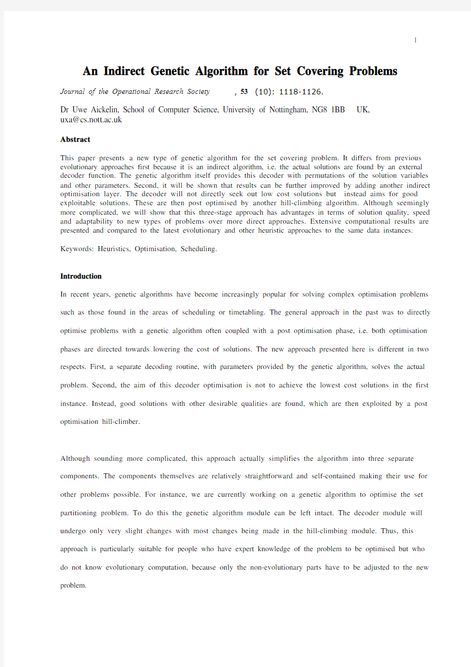
10个示例让你的VLOOKUP函数应用从入门到精通 VLOOKUP函数是众多的Excel用户最喜欢和最常用的函数之一,因此介绍VLOOKUP 函数使用技巧的文章也特别多。在《Excel函数学习4:VLOOKUP函数》中,我们学习了VLOOKUP函数的语法及应用,在Excel公式与函数之美前面的系列文章中,我们又详细探讨了VLOOKUP函数的4个参数。 熟练掌握VLOOKUP函数的使用,是Excel必备技能之一。下面我们通过10个示例,进一步巩固VLOOKUP函数的使用技能。 一键直达>> Excel函数学习4:VLOOKUP函数 一键直达>> Excel公式与函数之美15:VLOOKUP函数的秘密 一键直达>> Excel公式与函数之美19:理解VLOOKUP函数第4个参数的真实含义 一键直达>> Excel公式与函数之美20:MATCH函数使VLOOKUP函数更灵活高效 一键直达>> Excel公式与函数之美21:INDIRECT函数使VLOOKUP函数实现多表查询 一键直达>>Excel公式与函数之美22:VLOOKUP函数查找技巧 概述 VLOOKUP函数最擅长在列中查找相匹配的数据,若找到匹配的数据,则在找到的数据所在行的右边从指定的列中获取数据。 示例1:查找郭靖的数学成绩 如图1所示,在最左边的列中是学生的姓名,在列B至列E中是不同科目的成绩。
图1 现在,我需要从上面的数据中找到郭靖的数学成绩。公式为: =VLOOKUP("郭靖",$A$3:$E$10,2,0) 公式有4个参数: ?“郭靖”——要查找的值。 ?$A$3:$E$10——查找的单元格区域。注意,Excel在最左列搜索要查找的值,本例中在A3:A10中查找姓名郭靖。 ?2——一旦找到了郭靖,将定位到区域的第2列,返回郭靖所在行相同行的值。数值2指定从区域中的第2列查找成绩。 ?0——告诉VLOOKUP函数仅查找完全匹配的值。 以上面的示例来演示VLOOKUP函数是如何工作的。 首先,在区域的最左列查找郭靖,从顶部到底部查找并发现在单元格A7中存储着这个值。
indirect函数的使用方法 含义 此函数立即对引用进行计算,并显示其内容。当需要更改公式中单元格的引用,而不更改公式本身,请使用此函数,INDIRECT为间接引用。 语法 INDIRECT(ref_text,[a1]) Ref_text 为对单元格的引用,此单元格可以包含A1-样式的引用、R1C1-样式的引用、定义为引用的名称或对文本字符串单元格的引用。如果ref_text 不是合法的单元格的引用,函数INDIRECT 返回错误值#REF!或#NAME?。 如果ref_text 是对另一个工作簿的引用(外部引用),则工作簿必须被打开。如果源工作簿没有打开,函数INDIRECT 返回错误值#REF!。 a1 为一逻辑值,指明包含在单元格ref_text 中的引用的类型。 如果a1 为TRUE 或省略,ref_text 被解释为A1-样式的引用。 如果a1 为FALSE,ref_text 被解释为R1C1-样式的引用。 案例如下:
(案例一)工作簿内引用第一步 第二步
第三步 第四步
第五步 最终效果 (案例二)工作簿外引用 (1)步骤同案例一,只是引用在不同的sheet表里面 indirect(工作簿内).xlsx indirect(工作簿 外).xlsx indirect.xlsx
(2)老版excel用法 不同excel文件之间的引用案例 实例1 1:启动excel。 2:在Book1的Sheet1的单元格A1中键入“这是测试数据”。 在2003版及较早版的excel中,单击“文件”菜单上的“新建”,单击“工作簿”,然后点击“确定”。 3:在2007版中,单击按钮,单击“新建”,然后单击“创建”。 4:在Book2中,在Sheet1的单元格A1中键入Book1。 5:在Book2的Sheet1的单元格A2中键入Sheet1。 6:在Book2中,在Sheet1的单元格A3中键入A1。 7:保存这两个工作簿。 8:在2003版及较早版本的Excel中,在Book2的Sheet1的单元格B1中键入下面的公式:=INDIRECT(”’[“&A1&”.xls]”&A2&”’!”&A3) 在Excel 2007中,键入下面的公式: =INDIRECT(”’[“&A1&”.xls]”&A2&”’!”&A3) 该公式会返回“这是测试数据”。
用函数在Excel中从文本字符串提取数字 Excel输入数据过程中,经常出现在单元格中输入这样的字符串:GH0012JI、ACVB908、华升12-58JK、五香12.56元、0001#、010258等。在进行数据处理时,又需要把其中的数字0012、908、12-58、12.56、0001提取出来。 如何通过使用Excel的工作表函数,提取出字符串中的数字? 一、问题分析 对于已经输入单元格中的字符串,每一个字符在字符串中都有自己固定的位置,这个固定位置都可以用序列数(1、2、3、……)来表示,用这些序列数可以构成一个可用的常数数组。 以字符串“五香12.56元”为例:序列数1、2、3、4、5、6、7、8分别对应着字符串“五香12.56元”中字符“五”、“香”、“1”、“2”、“.”、“5”、“6”、“元”。由序列数组成一个保存在内存中的新数组{1;2;3;4;5;6;7;8}(用列的形式保存),对应字符串中的字符构成的数组{“五”;“香”;“1”;“2”;“.”;“5”;“6”;“元”}。因此解决问题可以从数组着手思考。 二、思路框架 问题的关键是,如何用序列数重点描述出字符串中的数字部分的起始位置和终止位置,从而用MID函数从指定位置开始提取出指定个数的字符(数字)。 不难看出,两个保存在内存中的新数组: {“五”;“香”;“ 1”;“2”;“.”;“5”;“6”;“元”} {1;2;3;4;5;6;7;8} 数组具有相同大小的数据范围,而后一个数组中的每一个数值可以准确地描述出字符串中字符位置。 字符与序列数的对应关系如下表所示: 字符字符位置
五—— 1 香—— 2 1 —— 3 2 —— 4 . —— 5 5 —— 6 6 —— 7 元—— 8 所以解决问题的基本框架是: 用MID函数从字符串的第一个数字位置起提取到最后一个数字止的字符个数。即{=MID(字符串,第一个数字位置,最后一个字符位置-第一个字符位置+1}。其中“+1”是补上最后一个数字位置减去第一个数字位置而减少的一个数字位。 三、解决方案及步骤 假定字符串输入在A2单元格。 ⑴确定A2中字符串的长度。 即用LEN函数计算出A2中字符串中字符的个数,这个字符个数值就是字符串中最后一个字符在字符串中的位置:=LEN(A2)。 ⑵确认字符串中的每一个字符位置序列数组成的新数组。 用INDIRECT函数返回一个由文本字符串指定的引用:
Excel函数公式使用心得 excel表格的基本操作在论坛学习已有时日,常见新手求助后兴奋地拿着答案回往了,可是题目解决了,却由于不能明白公式的含义,碰到类苏光目自己还难以举一反三应用甚至连一点小改动都需要再次求助;对函数公式略知一二者因不明公式含义不易拓展思路……等等现象,虽大多数都能在原帖得到热心版主、坛友的解答,屡见妙答,但没见到的人又重新发帖问及类苏光目,不利于各种题目的综合汇总,遂发此帖作为公式解释使用!一、怎样学习函数公式这是很多新手最想知道的事,函数那么多,要从哪儿学起呢。我个人谈点小体会:1、“学以致用”,用才是目的——就是你要和将要用到的东西先学。比如你根本用不上财务、工程函数,没必要一下子就往看那些专业性很强的东西(嘿嘿,那些我基本不会),这样就轻易进门了。基本上函数用得最多的逻辑判定和查找和引用这2类函数了。先不要急于学会“数组”,自己常用函数的普通用法有个大致的用法了解之后再往看它的数组用法。2、善于搜索,搜一下,能找到更多的解答;善于求助发帖求助要描述清楚附上必要的图文并茂的附件,轻易得到解答,而且锻炼了自己的表述能力。3、除了“求助”式学习,还要“助人”式的学习,相信这一点是众多论坛高手们都经历过的。只要有时间,
少看一会儿电视少聊一会儿QQ少跟同事吹一会儿牛,到论坛上看看有没有别人不懂而你懂的,别怕出糗,是驴是马牵出来遛遛,相信你热心帮人不会被嘲笑的,况窃冬抛砖引玉,说不定你抛的对别人甚至对高手来说也是块宝玉呢。而,助人助己,有了越来越多的“求助”者给你免费提供了练习的机会,练得多了再综合各种思路的比较,自己就有了一些想法,你的水平肯定与日俱增。4、一口气吃不成胖子,多记一些学习的体会,日积月累,你就是高手了。二、如何解读公式我也谈点小体会吧:1、多看函数帮助。各个函数帮助里面有函数的基本用法和一些“要点”,以及对数据排序、引用类型等等的要求。当然,函数帮助并不囊括所有函数的细微之处,不然,也就不会有那么多求“解释”的帖了。2、庖丁解牛——函数的参数之间用逗号隔开。(别笑话,这是最最基本的基本功,单个函数没啥,组合多个函数的公式就是靠它了),这些逗号就是“牛”的关节,先把长公式大卸八块之后逐个看明白了再拼凑起来读就轻易多了。3、独孤九剑——开个玩笑啦,这里是取谐音“F9键”。F9键用来“抹黑”公式对解读尤其是数组公式有非常强的作用,不过假如公式所含数据区域太大(比如上百行)你可以改变一下区域。具体方法比如下面这个简单数组公式 =sum(if(A1:A3>0,B1:B3)),用鼠标在编辑栏(或F2)把把A1:A3>0部分“抹黑”,按下F9键,就看到
了解Indirect 函数 返回由文本字符串指定的引用。此函数立即对引用进行计算,并显示其内容。当需要更改公式中单元格的引用,而不更改公式本身,请使用函数 INDIRECT。 前半句还好理解,后半句有点儿拗口了,其实大可不必在此深究这一句话的意思。个人觉得下面其他内容更重要。 语法 INDIRECT(ref_text,a1) Ref_text为对单元格的引用,此单元格可以包含 A1-样式的引用、R1C1-样式的引用、定义为引用的名称或对文本字符串单元格的引用。如果 ref_text 不是合法的单元格的引用,函数 INDIRECT 返回错误值 #REF!。 ?如果 ref_text 是对另一个工作簿的引用(外部引用),则那个工作簿必须被打开。如果源工作簿没有打开,函数 INDIRECT 返回错误值 #REF!。 ?如果 ref_text 引用的单元格区域超出行限制 1,048,576 或列限制 16,384 (XFD),则 INDIRECT 返回 #REF! 错误。注释此行为不同于 Microsoft Office Excel 2007 之前的 Excel 版本,早期的版本会忽略超出的限制并返 回一个值。 A1为一逻辑值,指明包含在单元格 ref_text 中的引用的类型。 ?如果 a1 为 TRUE 或省略,ref_text 被解释为 A1-样式的引用。 ?如果 a1 为 FALSE,ref_text 被解释为 R1C1-样式的引用。 ?第1参数要求 【示例文件】 通读完毕,其实看来INDIRECT很简单,就两个参数,一个是代表引用的字符串,一个是选择引用样式。 首先,我们选择熟悉的A1引用样式来解读,即默认使用一个参数或者第2参数为TRUE或非0数值: Ref_text为对单元格的引用,此单元格可以包含 A1-样式的引用、R1C1-样式的引用、定义为引用的名称或对文本字符串单元格的引用。如果 ref_text 不是合法的单元格的引用,函数 INDIRECT 返回错误值 #REF!。
查找与引用函数使用详解 1.ADDRESS 用途:以文字形式返回对工作簿中某一单元格的引用。 语法:ADDRESS(row_num,column_num,abs_num,a1,sheet_text) 参数:Row_num是单元格引用中使用的行号;Column_num是单元格引用中使用的列标;Abs_num指明返回的引用类型(1或省略为绝对引用,2绝对行号、相对列标,3相对行号、绝对列标,4是相对引用);A1是一个逻辑值,它用来指明是以A1或R1C1返回引用样式。如果A1为TRUE或省略,函数ADDRESS返回A1样式的引用;如果A1为FALSE,函数ADDRESS返回R1C1样式的引用。Sheet_text为一文本,指明作为外部引用的工作表的名称,如果省略sheet_text,则不使用任何工作表的名称。 实例:公式“=ADDRESS(1,4,4,1)”返回D1。 2.AREAS 用途:返回引用中包含的区域个数。 语法:AREAS(reference)。 参数:Reference是对某一单元格或单元格区域的引用,也可以引用多个区域。 注意:如果需要将几个引用指定为一个参数,则必须用括号括起来,以免Excel 将逗号作为参数间的分隔符。 实例:公式“=AREAS(a2:b4)”返回1,=AREAS((A1:A3,A4:A6,B4:B7,A16:A18))返回4。 3.CHOOSE 用途:可以根据给定的索引值,从多达29个待选参数中选出相应的值或操作。 语法:CHOOSE(index_num,value1,value2,...)。 参数:Index_num是用来指明待选参数序号的值,它必须是1到29之间的数字、或者是包含数字1到29的公式或单元格引用;value1,value2,...为1到29个数值参数,可以是数字、单元格,已定义的名称、公式、函数或文本。 实例:公式“=CHOOSE(2,"电脑","爱好者")返回“爱好者”。公式“=SUM(A1:CHOOSE(3,A10,A20,A30))”与公式“=SUM(A1:A30)”等价(因为CHOOSE(3,A10,A20,A30)返回A30)。 4.COLUMN
INDIRECT函数应用失败的实例分析及解决问题:INDIRECT("'"&$A2&"'!B2")这个公式是什么意思?为什么我同事的一个Excel表格用了INDIRECT的这个公式是可以的,我套用了却不行? 答复:INDIRECT函数 1、引用 B2=预先输入的内容!B2 很明显,该公式引用了工作表“预先输入的内容”中B2单元格的内容。本工作表B2单元格的值与预先输入的内容!B2的值相同。 2、地址 “A1”、“B2”分别表示一个单元格的地址,“预先输入的内容!B2”也表示一个单元格地址,是一个指定工作表的单元格地址。 如果预先知道单元格地址,在公式中使用该地址可以引用它的值。 3、文本 天安门广场是一个地址,把“天安门广场”写在纸片上,写在手心,它是一串文本,根据这个文本,向导可以把你带到天安门广场。文本和地址是两回事,不容易把它说清楚,但聪明的你可能已经心领神会了,OK。 4、转换 有了文本,需要向导才能到达,也一定能到达指定的地址。工作表中单元格地址也一样,“A1”与A1是两回事,“Sheet2!F7”与Sheet2!F7是两回事,知道地址文本,你要引用这个单元格的值,需要一个向导,它就INDIRECT()函数。 5、要点 要点之一:INDIRECT()函数的第一个参数为一个文本,一个表示单元格地址的文本。
要点之二:Excel对单元格有两种引用样式,一种为A1引用样式,一种为R1C1引用样式。当使用A1引用样式时,INDIRECT()函数第二个参数须指定为TRUE或省略它。当使用R1C1引用样式时,INDIRECT()的第二个参数须指定为FALSE。 INDIECT("F5"),与INDIRECT("F5",TRUE),与INDIRECT("R5C6",FALSE)返回同一个单元格的引用。 有朋友问,什么时候要用INDIRECT()?为什么要用INDIRECT()? 举个简单的例子: 如果B2:B10单元格分别要引用Sheet2:Sheet10工作表的F6单元格,则公式分别为:B2=Sheet2!F6 B3=Sheet3!F6 …… B10=Sheet10!F6 这些公式不能使用填充的办法输入,只能手工一个一个编辑修改。用什么办法可以快速填充?首行写入公式: B2="Sheet"&Row(2:2)&"!F6" 拖动填充柄把公式向下填充,依次得到结果: Sheet2!F6 Sheet3!F6 …… Sheet10!F6 但它显示的只是单元格地址,不是单元格引用。如果引用这些单元格的值? 在上面公式中,加入INDIRECT()函数就是: B2=INDIRECT("Sheet"&Row(2:2)&"!F6")
Excel中高级讲义 目录 一.公式基础 (2) 二.统计、文本基本函数 (4) 三.日期、信息基本函数 (4) 四.逻辑函数 (4) 五.数据查阅函数 (4) 六.常用快捷键 (5) 七.常用编辑命令 (5) 八.格式(format)··················································错误!未定义书签。 九.关于打印及其他 ·············································错误!未定义书签。 十.财务函数 ......................................................错误!未定义书签。十一.数据库操作 ...................................................错误!未定义书签。十二.数据引用 (6) 十三.选择性粘贴(paste special) (7) 十四.数据的有效性(validation) (8) 十五.数据的保护(protection)................................错误!未定义书签。十六.图表基础 ......................................................错误!未定义书签。十七.双轴图表 ......................................................错误!未定义书签。十八.保存自定义图表类型( custom chart type) ............错误!未定义书签。十九.分类汇总与合并计算 .......................................错误!未定义书签。二十.数据透视表 ...................................................错误!未定义书签。二十一.高级函数 (8) 二十二.高级筛选与数据库函数 ....................................错误!未定义书签。二十三.自定义格式 ...................................................错误!未定义书签。二十四.列表功能 (9) 二十五.导入外部数据(import extenal data) (9) 二十六.使用窗体控件(forms)···································错误!未定义书签。二十七.方案、单变量求解 ··········································错误!未定义书签。二十八.创建模拟运算表(table)·································错误!未定义书签。二十九.使用规划求解(solver) ····································错误!未定义书签。三十.数据的统计分析 ·············································错误!未定义书签。三十一.宏代码的录制与学习 ·······································错误!未定义书签。
INDIRECT 函数的语法及使用实例 INDIRECT 函数返回由文本字符串指定的引用。 什么情况下使用INDIRECT 函数? INDIRECT 函数返回由文本字符串指定的引用,可以用于:创建开始部分固定的引用;创建对静态命名区域的引用;从工作表、行、列信息创建引用;创建固定的数值组。 INDIRECT 函数语法 INDIRECT 函数函数的语法如下: INDIRECT(ref_text,a1) ref_text 是代表引用的文本字符串 如果a1为TRUE 或者忽略,使用A1引用样式;如果为FALSE ,使用R1C1引用样式 INDIRECT 陷阱 INDIRECT 函数 函数是易失的,因此如果在许多公式中使用,它会使工作簿变慢。 如果INDIRECT 函数 函数创建对另一个工作簿的引用,那么该工作簿必须打开,否则公式的结果为#REF!错误。 如果INDIRECT 函数创建所限制的行和列之外的区域的引用,公式将出现#REF!错误。(Excel 2007和Excel 2010) INDIRECT 函数不能对动态命名区域进行引用 2007 如果显示200V的话,这里v是7的意思,下面也一样
示例1:创建开始部分固定的引用 在第一个示例中,列C和列E有相同的数字,使用SUM函数求得的和也是相同的。然而,所使用的公式稍微有点不同。在单元格C8中,公式为:=SUM(C2:C7) 在单元格E8中,INDIRECT函数创建对开始单元格E2的引用: =SUM(INDIRECT(“E2″):E7) 如果在列表的顶部插入一行,例如输入January的数量,列C中的和不会改变,但公式发生了变化,根据被插入的行进行了调整: =SUM(C3:C8) 然而,INDIRECT函数锁定开始单元格为E2,因此January的数量被自动包括在E列的汇总单元格中。结束单元格改变,但是开始单元格没有受影响。 =SUM(INDIRECT(“E2″):E8)
解读INDIRECT函数 【帮助文件】解读 返回由文本字符串指定的引用。此函数立即对引用进行计算,并显示其内容。当需要更改公式中单元格的引用,而不更改公式本身,请使用函数 INDIRECT。 前半句还好理解,后半句有点儿拗口了,其实大可不必在此深究这一句话的意思。个人觉得下面其他内容更重要。 语法 INDIRECT(ref_text,a1) Ref_text为对单元格的引用,此单元格可以包含 A1-样式的引用、R1C1-样式的引用、定义为引用的名称或对文本字符串单元格的引用。如果 ref_text 不是合法的单元格的引用,函数 INDIRECT 返回错误值 #REF!。 ?如果 ref_text 是对另一个工作簿的引用(外部引用),则那个工作簿必须被打开。如果源工作簿没有打开,函数 INDIRECT 返回错误值 #REF!。 ?如果 ref_text 引用的单元格区域超出行限制 1,048,576 或列限制 16,384 (XFD),则 INDIRECT 返回 #REF! 错误。注释此行为不同于 Microsoft Office Excel 2007 之前的 Excel 版本,早期的版本会忽略超出的限制并返 回一个值。 A1为一逻辑值,指明包含在单元格 ref_text 中的引用的类型。 ?如果 a1 为 TRUE 或省略,ref_text 被解释为 A1-样式的引用。 ?如果 a1 为 FALSE,ref_text 被解释为 R1C1-样式的引用。 ?第1参数要求 【示例文件】 通读完毕,其实看来INDIRECT很简单,就两个参数,一个是代表引用的字符串,一个是选择引用样式。 首先,我们选择熟悉的A1引用样式来解读,即默认使用一个参数或者第2参数为TRUE或非0数值: Ref_text为对单元格的引用,此单元格可以包含 A1-样式的引用、R1C1-样式的引用、定义为引用的名称或对文本字符串单元格的引用。如果 ref_text 不是合法的单元格的引用,函数 INDIRECT 返回错误值 #REF!。 Ref在函数参数中一般指单元格引用;text则一般指字符串。这句话中,最重要的是告诉
实用EXCE的函数 用途:以文字形式返回对工作簿中某一单元格的引用。 语法:ADDRESS(row_num,column_num,abs_num,a1,sheet_text) 参数:Row_num是单元格引用中使用的行号;Column_num是单元格引用中使用的列标;Abs_num指明返回的引用类型(1或省略为绝对引用,2绝对行号、相对列标,3相对行号、绝对列标,4是相对引用);A1是一个逻辑值,它用来指明是以A1或R1C1返回引用样式。如果A1为TRUE或省略,函数ADDRESS返回A1样式的引用;如果A1为FALSE,函数ADDRESS返回R1C1样式的引用。Sheet_text为一文本,指明作为外部引用的工作表的名称,如果省略sheet_text,则不使用任何工作表的名称。 实例:公式“=ADDRESS(1,4,4,1)”返回D1。 用途:返回引用中包含的区域个数。 语法:AREAS(reference)。 参数:Reference是对某一单元格或单元格区域的引用,也可以引用多个区域。 注意:如果需要将几个引用指定为一个参数,则必须用括号括起来,以免Excel将逗号作为参数间的分隔符。
实例:公式“=AREAS(a2:b4)”返回1,=AREAS((A1:A3,A4:A6,B4:B7,A16:A18))返回4。 用途:可以根据给定的索引值,从多达29个待选参数中选出相应的值或操作。 语法:CHOOSE(index_num,value1,value2,...)。 参数:Index_num是用来指明待选参数序号的值,它必须是1到29之间的数字、或者是包含数字1到29的公式或单元格引用;value1,value2,...为1到29个数值参数,可以是数字、单元格,已定义的名称、公式、函数或文本。 实例:公式“=CHOOSE(2,"电脑","爱好者")返回“爱好者”。公式 “=SUM(A1:CHOOSE(3,A10,A20,A30))”与公式“=SUM(A1:A30)”等价(因为CHOOSE(3,A10,A20,A30)返回A30)。 用途:返回给定引用的列标。 语法:COLUMN(reference)。 参数:Reference为需要得到其列标的单元格或单元格区域。如果省略reference,则假定函数COLUMN是对所在单元格的引用。如果reference为一个单元格区域,并且函数COLUMN作为水平数组输入,则COLUMN函数将reference中的列标以水平数组的形式返回。
indirect函数的使用方法 excel中indirect函数,根据帮助,可以知道是返回并显示指定引用的内容。使用INDIRECT函数可引用其他工作簿的名称、工作表名称和单元格引用。 方法/步骤 indirect函数对单元格引用的两种方式。 看下图,使用indirect函数在C2、C3引用A1单元格的内容。 1、=INDIRECT("A1"),结果为C3。这种使用,简单的讲,就是将这些引用地址套上双引号,然后再传递给INDIRECT函数。 2、=INDIRECT(C1),结果为C2。解释:因为C1的值就是"A1",在公式编辑栏,选中“C1”,然后按下F9键,计算值,可以看到变为“"A1"”,本质没变,都是对单元格引用。 上面两者的区别在于:前者是A1单元格内文本的引用,后者是引用的C1单元格内的地址引用的单元格的内容。 indirect函数工作表名称的引用。 如果需要在“二班”工作表,计算“一班”工作表B2:B11的成绩总和。可以使用这样的公式:=SUM(INDIRECT("一班!B2:B11"))。解释:indirect(“工作表名!单元格区域”) 另外一种情况:当工作表名称直接是数字的,在工作表名称两边必须添加上一对单引号。
同样的,在“2”工作表,计算“1”工作表B2:B11的成绩总和。公式为:=SUM(INDIRECT("'1'!B2:B11"))。解释:indirect(“’工作表名’!单元格区域”)总结:如果工作表名为汉字,工作表名前后可以加上一对单引号,也可以不加。但是数字和一些特殊字符时,必须加单引号,否则不能得到正确结果。 我们在工作表命名时形成习惯尽量不要有空格和符号,这样可以不怕indirect引用忘记加单引号括起来。要么形成习惯所有indirect带工作表名引用时都用单引号将代表工作表名的字符串括起来。 INDIRECT函数对工作簿引用的书写方式和细节正确写法 =INDIRECT("[工作簿名.xls]工作表表名!单元格地址") INDIRECT函数,如果是对另一个工作簿的引用(外部引用),则那个工作簿必须被打开。如果源工作簿没有打开,函数INDIRECT 返回错误值#REF!。 Indirect函数应用实例一:制作多级下拉菜单 其原理是利用定义名称,然后在单元格输入与定义名称相同的字符再对含有这种字符的单元格用Indirect作引用。 未完待续……..
利用indirect函数的R1C1形式进行多表查 询汇总 多表查询汇总可以使用数据透视表进行,也可以使用导入外部数据结合sql 语句将各个表连接在一起进行汇总,如果只是做查询汇总,最高效和直观的方法是通过indirect函数实现的,这里用到两种嵌套函数的方式,其中第二种R1C1的形式是最容易理解的,也是最便捷的,在下面的实例中在设置完函数之后通过屏蔽零值,再利用条件格式设置非空单元格具有特定条件进一步完善查询汇总表。 方法/步骤 如下图显示的工作薄中有办公室、技术部、人力资源部、销售部四张工作表,每个表中存放的是各个部门的日常费用数据,包括日期、费用项目、金额、经办人这4个字段,现在需要根据不同的部门将各个字段对应的数据进行汇总为一张查询汇总表。
查询汇总表最终需要在b1单元格中选择部门,然后下方对应字段下会根据选择的部门自动将数据显示在汇总表中,此时选择部门对应的是办公室,可
以直接选中b4单元格,然后输入一个等号,然后点选办公室表中的a2单元格,然后将公式向下复制,但是如果这样操作,当部门名称发生变化时,下面的明细数据需要根据部门的变化发生变化。 如果使用index函数,首先需要将第一个参数通过点选设置为的a列,要取的行数在办公室表的第二行,而公式所在单元格为汇总表的第四行,所以可以将第二个参数设置为row()-2,作用是通过row函数算出当前单元格行号,然后减去2是因为在汇总表中比引用表中多了两行。
1. 4 在b1单元格中需要通过设置数据有效性来实现部门的选择,选中b1单元格,然后单击菜单栏数据命令,在弹出的菜单中点按有效性命令,在弹出的数据有效性对话框中选择设置选项卡,然后在允许下拉列表中选择序列,然后在来源中输入四个部门的名称用半角都好分隔开,然后点按确定,此时就可以通过技术部对应的下拉按钮来选择不同的部门了,作为查询依据的部门就可以按需要变动了。