
Supporting Direction Relations in Spatial Database Systems Yannis Theodoridis*Dimitris Papadias+Emmanuel Stefanakis*
*Department of Electrical and Computer Engineering National Technical University of Athens
Zographou, Athens, GREECE 15773
{theodor, stefanak}@theseas.ntua.gr +Department of Computer Science and Engineering University of California, San Diego
La Jolla, California, USA 92093-0114
dimitris@https://www.doczj.com/doc/b37325912.html,
Abstract Despite the attention that direction relations have attracted in domains such
as Spatial Query Languages, Image and Multimedia Databases, Reasoning and
Geographic Applications, they have not been extensively applied in spatial access
methods. In this paper we define direction relations between two-dimensional objects in
different levels of qualitative resolution and we show how these relations can be
efficiently retrieved in existing DBMSs using several indexing techniques. Then we
describe our implementations and provide experimental results on B- and R- tree-based
data structures to support direction relations efficiently.
Keywords: Direction relations, Spatial Data Structures, Query Optimisation.
1. INTRODUCTION
There has been an increasing interest recently about the representation and processing of spatial relations in Spatial Database Systems (for an extensive discussion see [Papa94c]). This interest has focused on several topics such as Reasoning [Fran95], Consistency Checking [Egen93] and Spatial Query Languages [Papa95a]. In this paper we deal with the retrieval of spatial relations in DBMSs used for geographic, or more generally, spatial, applications. In particular we concentrate on the retrieval of direction relations using B- and R- tree-based data structures.
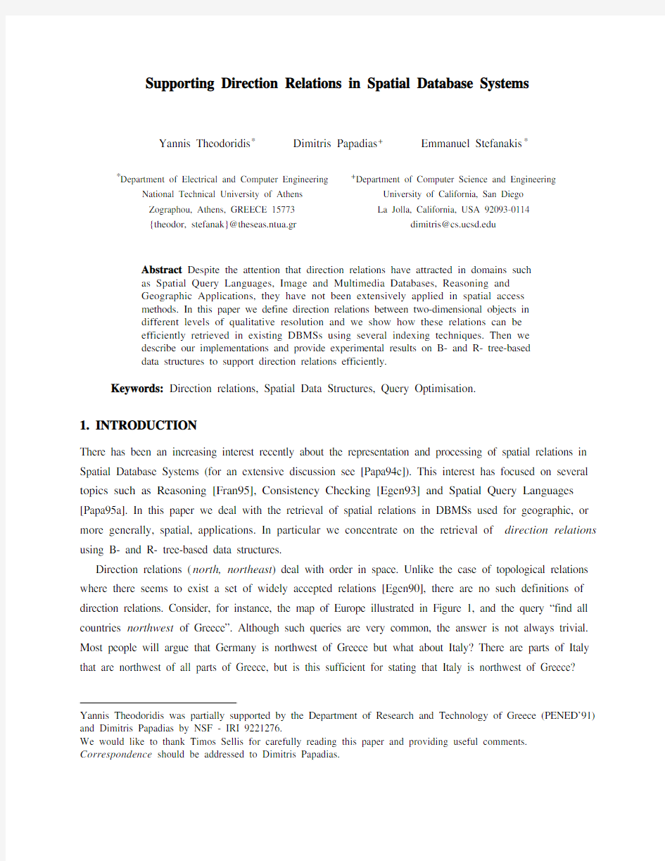
Direction relations (north, northeast) deal with order in space. Unlike the case of topological relations where there seems to exist a set of widely accepted relations [Egen90], there are no such definitions of direction relations. Consider, for instance, the map of Europe illustrated in Figure 1, and the query “find all countries northwest of Greece”. Although such queries are very common, the answer is not always trivial. Most people will argue that Germany is northwest of Greece but what about Italy? There are parts of Italy that are northwest of all parts of Greece, but is this sufficient for stating that Italy is northwest of Greece?
Yannis Theodoridis was partially supported by the Department of Research and Technology of Greece (PENED’91) and Dimitris Papadias by NSF - IRI 9221276.
We would like to thank Timos Sellis for carefully reading this paper and providing useful comments. Correspondence should be addressed to Dimitris Papadias.
Fig. 1 Map of Europe
The answer to this query depends on the definition of direction relations which may vary for each application. In this paper we define direction relations between two-dimensional objects in different levels of qualitative resolution to match the application needs. Our work extends previous attempts to formalise direction relations which have concentrated on point objects [Fran92, Papa94a] or Minimum Bounding Rectangles [Peuq87, Muke90]. Then we show how the relations that we define can be efficiently retrieved in existing DBMSs. Although for other types of spatial relations, such as topological relations, there has been extensive work in spatial data structures and specialised indexing methods have been proposed [Gutt84, Sell87, Beck90, Papa95b], limited work has focused on direction relations (see [Papa94b] for related work).
The results of this paper are directly applicable to Spatial Databases and Geographic Information Systems (GISs) where the formalization of spatial relations is crucial for user interfaces and query optimisation strategies. Furthermore, the importance of direction relations has been pointed out by several researchers in areas including Multimedia Databases [Sist94], Spatial Reasoning [Glas92], Cognitive Science [Jack83] and Linguistics [Hers86].
The paper is organised as follows. In section 2 we define several direction relations between objects in 2D-space. Section 3 describes how MBR approximations, commonly used in spatial access methods, can be used in the retrieval of direction relations. Sections 4 and 5 discuss the retrieval of direction relations using alternative access methods (B- and R- trees respectively). Section 6 is concerned with extensions to access methods that increase performance for some queries. Section 7 compares the different implementations illustrating experimental results, and section 8 concludes with comments on future work.
2. DIRECTION RELATIONS
In order to define direction relations between extended objects we first define relations between points and apply these definitions using universally and existentially quantified formulae. We assume an absolute frame of reference and a pair of orthocanonic axes x and y. Our method is projection based, that is, direction relations are defined using projection lines vertical to the coordinate axes. An alternative approach is based
on the cone-shaped concept of direction, i.e., direction relations are defined using angular regions between objects. Extensive studies of the two approaches can be found in [Fran95, Hern94].
For the following discussion p denotes the primary object (the object to be located) and q the reference object (the object in relation to which the primary object is located-in the following examples the reference object is grey). Let p i be a point of object p, q j be a point of object q, and X and Y be functions that give the x and y coordinate of a point. If we draw projection lines from a reference point, the plane is divided into nine partitions (Figure 2), each corresponding to one direction relation. The symbol * in Figure 2 illustrates the reference point (it also corresponds to the relation same_position ). ; T
< T \ QRUWKBZHVW UHVWULFWHGBZHVW VRXWKBZHVW [UHVWULFWHGBQRUWK QRUWKBHDVW
UHVWULFWHGBVRXWK
UHVWULFWHGBHDVW
VRXWKBHDVW Fig. 2 Plane partitions using one point per object
Some of the definitions for the relations of Figure 2 are given below, while the rest can be defined in the same way:
north_west(p i ,q j ) ≡ X(p i ) The above nine relations (including same_position ) correspond to the highest resolution that we can achieve when reasoning in terms of points using the concept of projections, in the sense that they cannot be represented as disjunctions of other relations. Exactly one of the previous relations holds true between any pair of points. The relations are transitive and same_position is also symmetric. The rest form four pairs of converse relations (e.g., north_east(p i ,q j ) ? south_west(q j , p i )). Additional direction relations can be defined using disjunctions of the nine relations; for example: north(p i ,q j ) ≡ north_west(p i ,q j ) ∨ restricted_north(p i ,q j ) ∨ north_east(p i ,q j ), south(p i ,q j ) ≡ south_west(p i ,q j ) ∨ restricted_south(p i ,q j ) ∨ south_east(p i ,q j ), same_level(p i ,q j ) ≡ restricted_west(p i ,q j ) ∨ same_position(p i ,q j ) ∨ restricted_east(p i ,q j ). Using the above definitions between points we can define spatial relations between objects. The relation strong_north between objects p and q, for instance, denotes that all points of p are north of all points of q:strong_north ≡ ?p i ?q j north(p i ,q j ), that is all points of the primary object must be in the shaded area (acceptance area) of Figure 3a. The relation strong_north can be characterised as low resolution relation because its acceptance area is large. On the other hand, we can define a higher resolution version of strong_north, as : strong_bounded_north(p,q) ≡ ?p i ?q j north(p i , q j ) ∧ ?p i ?q j north_east(p i , q j ) ∧ ?p i ?q j north_west(p i , q l ). According to this relation, all points of object p must be in the region bounded by the horizontal line that passes from q's northmost point and by the vertical lines that also bound q. For example,although Belgium is strong_north of Italy, it does not satisfy the relation strong_bounded_north because it is not in the shaded area of Figure 3b. (a)(b) Fig. 3 Acceptance area for strong_north and strong_bounded_north relations Table 1 illustrates several direction relations between objects using examples from the map of Figure 1.All of these relations concern the direction north, and they are representative for other relations as well, in the sense that they refer to several levels of qualitative resolution. Depending on the application needs, a large number of direction relations between extended objects can be defined and implemented accordingly. The set of direction relations can be chosen so that several properties are satisfied: the relations can be pairwise disjoint, provide a complete coverage, form a relation algebra etc. Notice that the relations that we study here do not satisfy any of these properties. The definition of pairwise disjoint relations is not a difficult task, but it is beyond the scope of this paper, which aims to show how direction relations of different resolution between extended objects can be defined and retrieved in spatial data structures. Furthermore, since the relations of Table 1 are concerned with direction north only,they do not provide a complete coverage. Customised direction relations between extended objects that satisfy the above properties and correspond to certain application needs are straightforward to develop using the definitions between points. Although the previous discussion refers to actual two-dimensional objects, usually spatial access methods store approximations that need only a few points for their representation, instead of the objects themselves.Such approximations are used to efficiently retrieve candidates that could satisfy a query. In this paper we examine methods based on the traditional approximation of Minimum Bounding Rectangles (MBRs). The next section discusses how MBRs can be used for the retrieval of direction relations between actual objects. 3. DIRECTION RELATIONS AND MINIMUM BOUNDING RECTANGLES Minimum Bounding Rectangles have been used extensively to approximate objects in Spatial Data Structures and Spatial Reasoning because they need only two points for their representation; in particular, each object q is represented as an ordered pair (q'l ,q'u ) of representative points that correspond to the lower left (q'l ) and the upper right point (q'u ) of the MBR q' that covers q. While MBRs demonstrate some disadvantages when approximating non convex or diagonal objects, they are the most commonly used approximations in spatial applications. Figure 4 illustrates how the map of Figure 1 can be approximated by MBRs.GR IT SP PO FR IR UK IC NO FI SW DE GE NL BE LU PL CZ RO BU AL YU CH AU HU Fig. 4 MBR approximations for the map of Europe Some access methods (e.g., R-trees) explicitly store MBRs, while others (e.g., B-trees) compare object locations using representative points. In order to answer the query “find all objects p that satisfy the relation R with respect to an object q” we have to retrieve all MBRs p' that satisfy the relation R' with respect to the MBR q' of object q. Table 1 illustrates the mapping from direction relations R between actual objects to relations R' between MBR representative points. Because MBRs differ from the actual objects they enclose, they are not always adequate to express the relation between the actual objects. For this reason, spatial queries involve the following two step strategy:First a filter step based on MBRs is used to rapidly eliminate MBRs of objects that could not possibly satisfy the query and select a set of potential candidates. Then during a refinement step each candidate is examined (by using computational geometry techniques) and false hits are detected and eliminated. Unlike topological relations, where the refinement step is the rule [Papa95b], the only direction relations of Table 1that need a refinement step are weak_bounded_north and weak_north_east [Papa94b]. For the rest of the relations all retrieved MBRs correspond to objects that satisfy the query. Table 1 Direction relations between objects and mapping to relations between MBRs In the next sections we will show how the above results can be applied to indexing techniques available in commercial DBMSs. The retrieval of direction relations in existing DBMSs could be accomplished by maintaining traditional indexes (e.g., B-trees1), or, alternatively, by incorporating Abstract Data Types (ADTs) with specialised indexes defined by external code (e.g., R-trees). Furthermore, when using extended-relational systems, like Postgres [Ston86], both indexing methods are available (or easily included) and application developers can decide which is the most appropriate for their application needs. 4. IMPLEMENTATION OF DIRECTION RELATIONS USING B-TREES The first solution for the retrieval of direction relations includes the maintenance of a group of 4 alphanumeric indexes, such as B-trees. Each index corresponds to one of the four numbers: p'l-x, p'l-y, p'u-x, p'u-, where p'l-x stands for the x-coordinate of the lower point of p', p'l-y for the y-coordinate of the lower point y and so on. Obviously, some relations imply search on one B-tree while others imply search on more B-trees. For instance, the query “find all objects p that are strong_north of object q” is transformed to the constraint north(p'l, q'u) or, in other words, p'l-y > q'u-y, which is a simple range query in the corresponding B-tree. On the other hand, other queries (such as strong_north_east) need to search two or more B-trees and, in a second phase, to compute the intersection of the intermediate answer sets. Table 2 presents the constraints needed for the retrieval of each direction relation using the set of four B-trees. Table 2 Constraints for the retrieval of direction relations using B-trees In general, the processing of a query of the form "find all objects p that satisfy a given direction relation with respect to object q" using B-trees involves the following steps: 1To be more precise, the implementation used in existing systems is the B+-tree index [Knut73] and, in this paper, we will think of B+-trees when we use the term B-trees. Step 1.Depending on the relation to be retrieved, select the B-trees involved from the set of four indexes. This procedure involves Table 2. Step 2.Search each index involved to find the corresponding answer sets. Step 3.If more than one index is involved, find the intersection set 2. Step 4.If necessary, follow a refinement step for the selected object IDs. As an example, consider the query: “Find the countries p strong_north_east of Switzerland (CH)”. In this case, two B-trees (for p'l-y and p'l-x parameters) need to be searched. They are illustrated in Figure 5a where each label indicates the appropriate coordinate for the corresponding object p, namely p'l-y and p'l-x . The sets {CZ', LU', BE', PL', UK', NL', IR', DE', SW', NO', FI', IC'} and {SW', CZ', PL', YU', HU', FI', RO', AL',GR', BU} are the two answer sets. The intersection set {CZ', PL', SW', FI'} contains the object IDs that satisfy the query (illustrated as the dark shaded area in Figure 3b). A refinement step is not needed for the retrieval of strong_north_east , that is, all retrieved MBRs correspond to objects that satisfy the query. (a) (b) Fig. 5 Retrieval of relation strong_north_east using B-trees The performance of the retrieval mechanism using B-trees depends significantly on the particular direction relation because the number of B-trees to be searched is equal to the number of constraints that are involved in the definition of the relation. Just_north , for example, involves only one exact matching constraint (p'l-y = q'u-y ), while weak_bounded_north contains four partial matching constraints (q'l-y < p'l-y 2A “realistic” assumption is that this procedure is executed in main memory. 5. IMPLEMENTATION OF DIRECTION RELATIONS USING R-TREES The R-tree data structure [Gutt84] is a height-balanced tree, which consists of intermediate and leaf nodes. The MBRs of the actual data objects are assumed to be stored in the leaf nodes of the tree. Intermediate nodes are built by grouping rectangles at the lower level. An intermediate node is associated with some rectangle which encloses all rectangles that correspond to lower level nodes. The fact that R-trees permit overlap among node entries sometimes leads to unsuccessful hits on the tree structure. The R+-tree [Sell87] and the R*-tree [Beck90] methods have been proposed to address the problem of performance degradation caused by the overlapping regions or excessive dead-space respectively. In this paper we use R*-trees because we found them to have consistently better performance in the retrieval of direction relations than both R- and R+- trees. In order to retrieve objects that satisfy a direction relation with respect to a reference object we have to specify the MBRs that could enclose such objects (Table 1) and then to search the intermediate nodes that contain these MBRs. Table 3 presents the constraints for the intermediate nodes for each direction relation of Table 1. Notice that the same relation between intermediate nodes and the reference MBR holds for all the levels of the tree structure. For instance, the intermediate nodes that could enclose other intermediate nodes P that satisfy the general constraint north(P u, q'u) should also satisfy the same constraint. This conclusion is applicable to all direction relations. Table 3 Constraints for intermediate nodes of R-trees In general, the processing of a query of the form "find all objects p that satisfy a given direction relation with respect to object q" using R-trees involves the following steps: Step 1.Starting from the top node, exclude the intermediate nodes P which could not enclose MBRs that satisfy the direction relation and recursively search the remaining nodes. This procedure involves Table 3. Step 2.Among the leaf nodes retrieved, select the ones that satisfy the direction relation. This procedure involves Table 1. Step 3.If necessary, follow a refinement step for the selected MBRs. Figure 6 shows how the MBRs of Figure 4 are grouped and stored in an R-tree. We assume a branching factor of 4, i.e., each intermediate node contains at most four entries. At the lower level MBRs of countries (denoted by two letters) are grouped into seven intermediate nodes A, B, C, D, E, F and G. At the next level,the seven nodes are grouped into two larger nodes X and Y. Consider now the query “Find the countries p strong_north_east of Switzerland (CH)”. The intermediate nodes that are selected for propagation are nodes X and Y (1st level), B, E, F and G (2nd level) i.e., the ones that have the representative point P u within the shaded area (these nodes are grey in the tree structure of Figure 6a). Among the leaves of the intermediate nodes B, E, F and G, the ones that satisfy the constraint north_east(p'l , CH'u ), are SW', FI', CZ' and PL'. (a)(b) Fig. 6 Retrieval of relation strong_north_east using R-trees Intuitively R-trees perform better than B-trees in cases where many constraints are involved in the definition of the direction relation of interest. The implementation of section 7 demonstrates that this is actually the case when four constraints are involved, while for one constraint B-trees have a better performance. For the intermediate relations though (two or three constraints) there is no clear winner and modified versions of the two data structures can yield better results. In the next section we present extensions of B-trees and R -trees that facilitate efficiency for some types of queries. 6. EXTENSIONS OF B-TREES AND R-TREES In the case of B-trees, we propose schemes for the maintenance of information regarding the MBR extents in the index; we call the proposed structures composite B-trees . As shown in section 4, the number of B-trees to be searched is equal to the number of constraints that compose the query. This inconvenience may be overcome if the B-tree accommodates additional information regarding the MBRs in its leaf nodes . That is, a composite key may be maintained instead of a simple numerical value (i.e., the coordinate value of one MBR corner). This composite key consists of the coordinate values of the two MBR corners in one axis (x- or y-axis) or even of all four coordinates of the two MBR corners. One of these coordinates is the primary component, and based on its value the B-tree is built. The rest of the coordinates are used for the elimination of irrelevant MBRs. The key of the composite B-tree considered here consists of two values that represent the lower and upper coordinates of each MBR in one of the two axes. One of these values is the primary component. This scheme reduces each MBR into two line segments which represent its extents over the two dimensions of the space and are indexed separately. Clearly, the efficient retrieval of direction relations can be achieved when four composite B-trees are maintained: B l-x-tree that keeps p'l-x as primary component and p'u-x as secondary component, and, similarly, B u-x-tree, B l-y-tree and B u-y-tree. Some relations imply the search of only one B-tree (such as strong_north), while the rest imply exactly two searches (i.e., one for each axis such as strong_north_east). In addition, provided that the information regarding the MBRs' extents over each axis are maintained in two indices, the approach to satisfy a query is not unique. For instance, relation weak_north requires no index to be searched for the x-axis, but it may be satisfied by searching either a B l-y-tree (condition to be fulfilled: q'l-y< p'l-y< q'u-y; refinement condition: p'u-y > q'u-y) or a B u-y-tree (condition to be fulfilled: p'u-y > q'u-y; refinement condition: q'l-y< p'l-y< q'u-y). The processing of a direction relation query involves the four steps described in section 4. During step 2 the search of each index is based on the primary component of the composite key while, in the leaf nodes, the possible refinement condition for the secondary component is considered to eliminate irrelevant MBRs. The selection of the most effective B-tree by a query processor or optimiser is not always trivial. In general, the selection should take into account: a) the direction relation involved; b) the query window size and position; and c) the distribution of MBR corners over the work space (this depends on the MBRs distribution and size). We propose three schemes for the selection of the most effective B-tree: ? Selection based on the relation involved: This scheme selects the index based on the relation using statistical results. For example, the B l-y-tree is chosen for strong_north and (arbitrarily for) north_south relations. ? Selection based on the location and size of the query object: The query object divides each axis of the work space into five ranges: A = (-∞,q l); B = q l; C = (q l,q u); D = q u; E = (q u,+∞). This scheme assumes that the MBR corners are uniformly distributed over the work space and selects the index based on the shortest range or sum of ranges involved. For example, the B l-y-tree is chosen for north_south relation only if range A is shorter that range E; otherwise the B u-y-tree is chosen. ? Selection based on the location and size of the query object and the distribution of MBR corners: This scheme may select the most effective index. This is obtained by maintaining an array (directory) with information about the number of lower and upper coordinates over the work space using a pre-determined resolution. For a given query object the lower and upper coordinates that fall within the five ranges A, B, C, D and E are computed, so that the number of segments to be retrieved for the two candidate indices is derived. The composite B-tree with the fewest segments is then chosen. The three schemes have been implemented and tested (see [Stef95] for detailed experimental results). As a general conclusion, the third scheme outperforms the other two schemes. The second scheme may provide an improvement in performance when the data set consists of small MBRs and, as a consequence, the assumption of the uniform distribution of MBR corners over the space is true. On the other hand, R-trees handle two-dimensional data efficiently when the search procedure involves both axes of the work space. However, several direction relations, such as strong_north, north_south, etc., involve search on only one axis. In such cases, the information regarding the other axis, which is maintained in the two-dimensional R-tree is useless. Clearly, a one-dimensional R-tree (i.e., segment tree), which is an index of the MBR extents along the axis of interest, would be more efficient because it is more compact (tree nodes accommodate a larger number of entries) and effective (the MBR extents along the other axis do not affect the maintenance of the index) than the two-dimensional R-tree. To obtain a more efficient retrieval of direction relations that involve only one axis of the space, two one-dimensional R-trees are needed to index the MBR extents over each axis separately. The set of the two trees can also support the retrieval of direction relations that involve both axes, such as strong_north_east. Each index provides a set of MBRs, and the intersection of the two sets composes the qualified set. In such cases though, the two-dimensional R-tree is expected to be more efficient. After the description of the alternative implementations of direction relations in practical systems using several indexing techniques we compare the efficiency of retrieval. It is not easy to claim a-priori which solution is the best for each direction relation but it is more sensible to claim that particular structures are more suitable for some queries. 7. PERFORMANCE COMPARISON In the previous sections we have argued that the performance of each procedure depends significantly on the particular direction relation. In this section we present several experimental results that justify our argument. In order to experimentally quantify the performance, we created tree structures by inserting 10000 randomly generated MBRs. We tested three data files: -the first file contains small MBRs: the size of each rectangle is at most 0.02% of the global area -the second file contains medium MBRs: the size of each rectangle is at most 0.1% of the global area -the third file contains large MBRs: the size of each rectangle is at most 0.5% of the global area. The search procedure used three query files for each data file containing 100 rectangles, also randomly generated, with similar size properties as the data rectangles. We used the previous data files for the retrieval of direction relations in classic B-trees, composite B-trees, 2D R-trees and 1D R-trees. The performance of each structure per relation (for each data / query size combination) is illustrated in Figure 7. Fig. 7 Performance Comparison As a first conclusion we notice the way that the data and query size affect the performance of the data structures. The performance of B-trees depends significantly on the query size while the opposite happens for R-trees where the data size is the main factor responsible for the high or low performance of the structure. The main results extracted by Figure 7 are the following: ? The classic B-tree is the most efficient structure for 1-constraint relations only (e.g., strong_north, just_north). In that case the classic B-tree outperforms even the (dedicated) composite B-tree because of its higher compactness3.When more constraints (even for the same axis) are involved it is not competitive.? The composite B-tree is the most efficient method for large data when more than one constraint is involved (e.g., weak_north and weak_bounded_north for large data files), since R-trees are unable to index such data efficiently. On the other hand, it is sensitive to query size; large queries are not handled efficiently by composite B-trees. ? The two-dimensional R-tree is the winner when three or four constraints are involved (see strong_bounded_north, weak_bounded_north), assuming that data rectangles are not large. In such cases, R-trees are not able to organise the data efficiently. ? The one-dimensional R-tree is the winner when two constraints along the same axis are involved (see weak_north relation), with the exception of large data files because of the reason mentioned above. From the above results, it is evident that there is not an overall winner but the performance of the structures is affected significantly by the number of constraints involved, the size of the data rectangles and the query size. However, the above results can be used as guidelines to spatial query processors and optimisers in order to select appropriate indexes for use in answering spatial queries. 8. CONCLUSION This paper describes implementations of direction relations in Spatial DBMSs. Direction relations constitute a new type of query for spatial access methods which so far have been concerned with disjoint/overlap relations [Same89], topological relations of high resolution [Papa95b] and distance relations such as nearest neighbour queries [Rous95]. Despite the fact that direction queries are of equal importance to previous ones they have not been extensively implemented, mainly because of the lack of well-defined direction relations between actual objects. In this work we define direction relations between points and we use these definitions as a basis for relations between objects. For the purposes of this paper we use a set of eight object relations, but a large number of additional ones can be defined using the point relations. Then we show how these relations can be retrieved in existing DBMSs using B-trees and R-trees. We also propose extensions of these data structures, called composite B-trees and 1D R-trees, to facilitate efficiency for some types of queries. 3The capacity of leaf-nodes in the classic B-tree is 126 keys while composite B-trees keep 84 keys in the leaf-nodes. For the implementation of the proposed techniques we used data and query files of different sizes. The main conclusion that arises from the experimental comparison of the alternative techniques is that there is not a data structure that performs better in all queries but the performance depends on the following factors: 1. the number and the type of constraints involved in the definition of the direction relations of interest 2. the data size (i.e., the size of the primary MBRs) 3. the query size (i.e., the size of the reference MBRs) It is possible that in actual systems, two or more of the previous structures can be used alternatively in conjunction with an optimiser that chooses the most suitable one according to the input query. Future work can be done on the definition and implementation of direction relations. Experimental findings from Cognitive and Environmental Psychology4 can be used as guidelines for the direction relations that people evoke in everyday reasoning. Although so far the psychological results are too vague to be helpful in defining direction relations in actual systems, ongoing research can lead to a set of well defined and psychologically sound relations. Note that such a set exists for topological relations [Egen90]. Progress can also be achieved in specialised data structures that have a better performance for queries involving direction relations or combinations of several types of spatial information (e.g., “find the five closest buildings in the area northeast of the (burning) factory”. REFERENCES [Beck90]Beckmann, N., Kriegel, H.P., Schneider, R., Seeger, B., “The R*-tree: an Efficient and Robust Access Method for Points and Rectangles”, In the Proceedings of ACM-SIGMOD Conference, 1990. [Egen90]Egenhofer, M., Herring, J., “A Mathematical Framework for the Definitions of Topological Relationships”, In the Proceedings of the 4th International Symposium on Spatial Data Handling (SDH), 1990. [Egen93]Egenhofer, M., Sharma, J., “Assessing the Consistency of Complete and Incomplete Topological Information”, Geographical Systems, Vol. 1, pp. 47-68, 1993. [Fran92]Frank, A.U., “Qualitative Spatial Reasoning about Distances and Directions in Geographic Space”, Journal of Visual Languages and Computing, Vol. 3, pp. 343-371, 1992. [Fran95]Frank, A.U., “Qualitative Spatial Reasoning: Cardinal Directions as an Example”, to appear in the International Journal of Geographic Information Systems. [Glas92]Glasgow, J.I., Papadias, D., “Computational Imagery”, Cognitive Science, Vol. 16, pp. 355-394, 1992. [Gutt84]Guttman, A., “R-trees: a Dynamic Index Structure for Spatial Searching”, In the Proceedings of ACM-SIGMOD Conference, 1984. [Hern94]Hernandez, D., “Qualitative Representation of Spatial Knowledge”, Springer Verlag LNAI, 1994. [Hers86]Herskovits, A., “Language and Spatial Cognition”, Cambridge University Press, 1986. [Jack83]Jackendoff, R., “Semantics and Cognition”, MIT Press, 1983 4A survey and an experimental study regarding the use of direction relations in cognitive spatial reasoning at geographic scales can be found in [Mark92]. [Knut73]Knuth, D., “The Art of Computer Programming, vol 3: Sorting and Searching”, Addison-Wesley, 1973. [Mark92]Mark, D., “Counter-Intuitive Geographic 'Facts': Clues for Spatial Reasoning at Geographic Scales”, In the Proceedings of International Conference GIS - From Space to Territory: Theories and Methods of Spatio-Temporal Reasoning in Geographic Space, 1992. [Muke90]Mukerjee, A., Joe, G., “A Qualitative Model for Space”, Technical Report TAMU 90-005, Texas A&M University, 1990. [Papa94a]Papadias, D., Frank, A.U., Koubarakis, M., “Constraint-Based Reasoning in Geographic Databases: The Case of Symbolic Arrays”, In the Proceedings of the 2nd ICLP Workshop on Deductive Databases, 1994. [Papa94b]Papadias, D., Theodoridis, Y., Sellis, T., “The Retrieval of Direction Relations Using R-trees”, In the Proceedings of the 5th Conference on Database and Expert Systems Applications (DEXA), 1994. [Papa94c]Papadias, D., Sellis, T., “The Qualitative Representation of Spatial Knowledge in two-dimensional Space”, Very Large Data Bases Journal, Special Issue on Spatial Databases, Vol 3(4), pp. 479-516, 1994. [Papa95a]Papadias, D., Sellis, T., “A Pictorial Query-by-Example Language”, to appear in the Journal of Visual Languages and Computing, Special issue on Visual Query Systems. [Papa95b]Papadias, D., Theodoridis, Y., Sellis, T., Egenhofer, M., “Topological Relations in the World of Minimum Bounding Rectangles: a Study with R-trees”, In the Proceedings of ACM-SIGMOD Conference, 1995. [Peuq87]Peuquet, D., Ci-Xiang, Z., “An Algorithm to Determine the Directional Relationship between Arbitrarily-Shaped Polygons in the Plane”, Pattern Recognition, Vol. 20(1), 1987, pp. 65-74. [Rous95]Roussopoulos, N., Kelley, F., Vincent, F., “Nearest Neighbor Queries”, In the Proceedings of ACM-SIGMOD Conference, 1995. [Same89]Samet, H., “The Design and Analysis of Spatial Data Structures”, Addison-Wesley, 1989. [Sell87]Sellis, T., Roussopoulos, N., Faloutsos, C., “The R+-tree: A Dynamic Index for Multi-Dimensional Objects”, In the Proceedings of the 13th Very Large Data Bases Conference, 1987. [Stef95]Stefanakis, E., Theodoridis, Y., “B-trees and Spatial Relations in Two-Dimensional Space”, Technical Report, KDBSLAB-TR-95-01, National Technical University of Athens, 1995. [Ston86]Stonebraker, M., Rowe, L., “The Design of Postgres”, In the Proceedings of ACM-SIGMOD Conference, 1986. [Sist94]Sistla, P., Yu, C., Haddad, R., “Reasoning about Spatial Relationships in Picture Retrieval Systems”, In the Proceedings of the 20th Very Large Data Bases Conference, 1994. STC89C52是一种带8K字节闪烁可编程可檫除只读存储器(FPEROM-Flash Programable and Erasable Read Only Memory )的低电压,高性能COMOS8的微处理器,俗称单片机。该器件采用ATMEL 搞密度非易失存储器制造技术制造,与工业标准的MCS-51指令集和输出管脚相兼容。 单片机总控制电路如下图4—1: 图4—1单片机总控制电路 1.时钟电路 STC89C52内部有一个用于构成振荡器的高增益反相放大器,引 脚RXD和TXD分别是此放大器的输入端和输出端。时钟可以由内部方式产生或外部方式产生。内部方式的时钟电路如图4—2(a) 所示,在RXD和TXD引脚上外接定时元件,内部振荡器就产生自激振荡。定时元件通常采用石英晶体和电容组成的并联谐振回路。晶体振荡频率可以在1.2~12MHz之间选择,电容值在5~30pF之间选择,电容值的大小可对频率起微调的作用。 外部方式的时钟电路如图4—2(b)所示,RXD接地,TXD接外部振荡器。对外部振荡信号无特殊要求,只要求保证脉冲宽度,一般采用频率低于12MHz的方波信号。片内时钟发生器把振荡频率两分频,产生一个两相时钟P1和P2,供单片机使用。 示,RXD接地,TXD接外部振荡器。对外部振荡信号无特殊要求,只要求保证脉冲宽度,一般采用频率低于12MHz的方波信号。片内时钟发生器把振荡频率两分频,产生一个两相时钟P1和P2,供单片机使用。 RXD接地,TXD接外部振荡器。对外部振荡信号无特殊要求,只要求保证脉冲宽度,一般采用频率低于12MHz的方波信号。片内时钟发生器把振荡频率两分频,产生一个两相时钟P1和P2,供单片机使用。 STC89C52RC单片机介绍 STC89C52RC单片机是宏晶科技推出的新一代高速/低功耗/超强抗干扰的单片机,指令代码完全兼容传统8051单片机,12时钟/机器周期和6时钟/机器周期可以任意选择。 主要特性如下: 增强型8051单片机,6时钟/机器周期和12时钟/机器周期可以任意选择,指令代码完全兼容传统8051. 工作电压:~(5V单片机)/~(3V单片机) 工作频率范围:0~40MHz,相当于普通8051的0~80MHz,实际工作频率可达48MHz 用户应用程序空间为8K字节 片上集成512字节RAM 通用I/O口(32个),复位后为:P1/P2/P3/P4是准双向口/弱上拉,P0口是漏极开路输出,作为总线扩展用时,不用加上拉电阻,作为 I/O口用时,需加上拉电阻。 ISP(在系统可编程)/IAP(在应用可编程),无需专用编程器,无需专用仿真器,可通过串口(RxD/,TxD/)直接下载用户程序,数秒 即可完成一片 具有EEPROM功能 具有看门狗功能 共3个16位定时器/计数器。即定时器T0、T1、T2 外部中断4路,下降沿中断或低电平触发电路,Power Down模式可由外部中断低电平触发中断方式唤醒 通用异步串行口(UART),还可用定时器软件实现多个UART 工作温度范围:-40~+85℃(工业级)/0~75℃(商业级) PDIP封装 STC89C52RC单片机的工作模式 掉电模式:典型功耗<μA,可由外部中断唤醒,中断返回后,继续执行 原程序 空闲模式:典型功耗2mA 正常工作模式:典型功耗4Ma~7mA 掉电模式可由外部中断唤醒,适用于水表、气表等电池供电系统及便携设备 STC89C52RC引脚图 STC89C52RC引脚功能说明 VCC(40引脚):电源电压 VSS(20引脚):接地 P0端口(~,39~32引脚):P0口是一个漏极开路的8位双向I/O口。作为输出端口,每个引脚能驱动8个TTL负载,对端口P0写入“1”时,可以作为高阻抗输入。 STC89C52单片机用户手册 [键入作者姓名] [选取日期] STC89C52RC单片机介绍 STC89C52RC单片机是宏晶科技推出的新一代高速/低功耗/超强抗干扰的单片机,指令代码完全兼容传统8051单片机,12时钟/机器周期和6时钟/机器周期可以任意选择。 主要特性如下: 1.增强型8051单片机,6时钟/机器周期和12时钟/机器周期可以任 意选择,指令代码完全兼容传统8051. 2.工作电压:5.5V~ 3.3V(5V单片机)/3.8V~2.0V(3V单片机) 3.工作频率范围:0~40MHz,相当于普通8051的0~80MHz,实 际工作频率可达48MHz 4.用户应用程序空间为8K字节 5.片上集成512字节RAM 6.通用I/O口(32个),复位后为:P1/P2/P3/P4是准双向口/弱上 拉,P0口是漏极开路输出,作为总线扩展用时,不用加上拉电阻, 作为I/O口用时,需加上拉电阻。 7.ISP(在系统可编程)/IAP(在应用可编程),无需专用编程器,无 需专用仿真器,可通过串口(RxD/P3.0,TxD/P3.1)直接下载用 户程序,数秒即可完成一片 8.具有EEPROM功能 9.具有看门狗功能 10.共3个16位定时器/计数器。即定时器T0、T1、T2 11.外部中断4路,下降沿中断或低电平触发电路,Power Down模式 可由外部中断低电平触发中断方式唤醒 12.通用异步串行口(UART),还可用定时器软件实现多个UART 13.工作温度范围:-40~+85℃(工业级)/0~75℃(商业级) 14.PDIP封装 STC89C52RC单片机的工作模式 ●掉电模式:典型功耗<0.1μA,可由外部中断唤醒,中断返回后,继续执行原 程序 ●空闲模式:典型功耗2mA ●正常工作模式:典型功耗4Ma~7mA ●掉电模式可由外部中断唤醒,适用于水表、气表等电池供电系统及便携设备 STC89C52单片机学习开发板介绍 全套配置: 1 .全新增强STC89C5 2 1个【RAM512字节比AT89S52多256个字节FLASH8K】 2 .优质USB数据线 1条【只需此线就能完成供电、通信、烧录程序、仿真等功能,简洁方便实验,不需要USB 转串口和串口线,所有电脑都适用】 3 .八位排线 4条【最多可带4个8*8 LED点阵,从而组合玩16*16的LED点阵】 4 .单P杜邦线 8条【方便接LED点阵等】 5 .红色短路帽 19个【已装在开发箱板上面,短路帽都是各功能的接口,方便取用】 6 .实验时钟电池座及电池 1PCS 7 .DVD光盘 1张【光盘具体内容请看页面下方,光盘资料截图】 8 .全新多功能折叠箱抗压抗摔经久耐磨 1个【市场没有卖,专用保护您爱板的折叠式箱子,所有配件都可以放入】 9 .8*8(红+绿)双色点阵模块 1片【可以玩各种各样的图片和文字,两种颜色变换显示】 10.全新真彩屏SD卡集成模块 1个【请注意:不包含SD卡,需要自己另外配】 晶振【1个方便您做实验用】 12.全新高速高矩进口步进电机 1个【价格元/个】 13.全新直流电机 1个【价值元/ 个】 14.全新红外接收头 1个【价格元/ 个】 15.全新红外遥控器(送纽扣电池) 1个【价格元/个】 16.全新18B20温度检测 1个【价格元/只】 17.光敏热敏模块 1个(已经集成在板子上)【新增功能】 液晶屏 1个 配件参照图: 温馨提示:四点关键介绍,这对您今后学习51是很有帮助的) 1.板子上各模块是否独立市场上现在很多实验板,绝大部分都没有采用模块化设计,所有的元器件密 密麻麻的挤在一块小板上,各个模块之间PCB布线连接,看上去不用接排线,方便了使用者,事实上是为了降低硬件成本,难以解决各个模块之间的互相干扰,除了自带的例程之外,几乎无法再做任何扩展,更谈不上自由组合发挥了,这样对于后继的学习非常不利。几年前的实验板,基本上都是这种结构的。可见这种设计是非常过时和陈旧的,有很多弊端,即便价格再便宜也不值得选购。 HC6800是采用最新设计理念,实验板各功能模块完全独立,互不干扰,功能模块之间用排线快速连接。 一方面可以锻炼动手能力,同时可加强初学者对实验板硬件的认识,熟悉电路,快速入门;另一方面,因为各功能模块均独立设计,将来大家学习到更高级的AVR,PIC,甚至ARM的时候,都只 STC89C52RC 单片机介绍 STC89C52RC 单片机是宏晶科技推出的新一代高速/低功耗/超强抗干扰的单片机,指令代码完全兼容传统8051 单片机,12 时钟/机器周期和 6 时钟/机器周期可以任意选择。 主要特性如下: 1. 增强型8051 单片机,6 时钟/机器周期和12 时钟/机器周期可以任意选择,指令代码完全兼容传统 8051. 2. 工作电压:5.5V~ 3.3V<5V 单片机)/3.8V~2.0V<3V 单片机) 3. 工作频率范围:0~40MHz,相当于普通 8051 的 0~80MHz,实际工作频率可达 48MHz 4. 用户应用程序空间为 8K 字节 5. 片上集成 512 字节 RAM 6. 通用I/O 口<32 个)复位后为:,P1/P2/P3/P4 是准双向口/弱上拉,P0 口是漏极开路输出,作为总线扩展用时,不用加上拉电阻,作为I/O 口用时,需加上拉电阻。 7. ISP<在系统可编程)/IAP<在应用可编程),无需专用编程器,无需专用仿真器,可通过串口 STC89C52F单片机介绍 STC89C52F单片机是宏晶科技推出的新一代高速 /低功耗/超强抗干扰的单片机,指令代码完全兼容传统8051单片机,12时钟/机器周期和6时钟/机器周期可以任意选择。 主要特性如下: * 增强型8051单片机,6时钟/机器周期和12时钟/机器周期可以任意选择,指令代码完全兼容传统8051. * 工作电压:5.5V?3.3V (5V单片机)/3.8V?2.0V (3V单片机) * 工作频率范围:0?40MHz相当于普通8051的0?80MHz实际工作频率可达48MHz *用户应用程序空间为8K字节 * 片上集成512字节RAM * 通用I/O 口(32个),复位后为:P1/P2/P3/P4是准双向口 /弱上拉,P0 口是漏极开路输出,作为总线扩展用时,不用加上拉电阻,作为I/O 口 用时,需加上拉电阻。 * ISP (在系统可编程)/IAP (在应用可编程),无需专用编程器,无需专用仿真器,可通过串口( RxD/P3.0,TxD/P3.1 )直接下载用户程序,数秒 即可完成一片 * 具有 EEPROM能 *具有看门狗功能 * 共3个16位定时器/计数器。即定时器T0、T1、T2 * 外部中断4路,下降沿中断或低电平触发电路,Power Down模式可由外部中断低电平触发中断方式唤醒 * 通用异步串行口( UART,还可用定时器软件实现多个 UART * 工作温度范围:-40?+85C(工业级)/0?75C(商业级) * PDIP封装 STC89C52F单片机的工作模式 *掉电模式:典型功耗<0.1吩,可由外部中断唤醒,中断返回后,继续执行原程序 STC89C52 单片机介绍: 单片机是指一个集成在一块芯片上的完整计算机系统。尽管他的大部分功能集成在一块小芯片上,但是它具有一个完整计算机所需要的大部分部件:CPU、内存、内部和外部总线系统,目前大部分还会具有外存。同时集成诸如通讯接口、定时器,实时时钟等外围设备。而现在最强大的单片机系统甚至可以将声音、图像、网络、复杂的输入输出系统集成在一块芯片上。 单片机也被称为微控制器(Microcontroler),是因为它最早被用在工业控制领域。单片机由芯片内仅有CPU的专用处理器发展而来。最早的设计理念是通过将大量外围设备和CPU集成在一个芯片中,使计算机系统更小,更容易集成进复杂的而对提及要求严格的控制设备当中。INTEL的Z80是最早按照这种思想设计出的处理器,从此以后,单片机和专用处理器的发展便分道扬镳。 早期的单片机都是8位或4位的。其中最成功的是INTEL的8031,因为简单可靠而性能不错获得了很大的好评。此后在8031上发展出了MCS51系列单片机系统。基于这一系统的单片机系统直到现在还在广泛使用。随着工业控制领域要求的提高,开始出现了16位单片机,但因为性价比不理想并未得到很广泛的应用。90年代后随着消费电子产品大发展,单片机技术得到了巨大的提高。随着INTEL i960系列特别是后来的ARM系列的广泛应用,32位单片机迅速取代16位单片机的高端地位,并且进入主流市场。而传统的8位单片机的性能也得到了飞速提高,处理能力比起80年代提高了数百倍。目前,高端的32位单片机主频已经超过300MHz,性能直追90年代中期的专用处理器,而普通的型号出厂价格跌落至1美元,最高端的型号也只有10美元。当代单片机系统已经不再只在裸机环境下开发和使用,大量专用的嵌入式操作系统被广泛应用在全系列的单片机上。而在作为掌上电脑和手机核心处理的高端单片机甚至可以直接使用专用的Windows和Linux操作系统。 单片机比专用处理器更适合应用于嵌入式系统,因此它得到了最多的应用。事实上单片机是世界上数量最多的计算机。现代人类生活中所用的几乎每件电子和机械产品中都会集成有单片机。手机、电话、计算器、家用电器、电子玩具、掌上电脑以及鼠标等电脑配件中都配有1-2部单片机。而个人电脑中也会有为数不少的单片机在工作。汽车上一般配备40多部单片机,复杂的工业控制系统上 3.2 51单片机部分 3.2.1 单片机选型依据 MCS-51系列为美国Intel公司在上世纪80年代推出的一种8位单片机。在芯片的集成程度上有较大提高,同时也大幅提升了性能,单片机的功能也大大丰富,功能单元的数量与种类答复增加,取得巨大成功,如今在我国获得广泛的应用。 MMCS51单片机的内部总体结构其基本特性如下: 8位CPU、片内振荡器、4k字节ROM、128字节RAM、21个特殊功能寄存器、32根I/O线、可寻址的64k字节外部数据、程序存贮空间、2个16位定时器、计数器中断结构:具有二个优先级、五个中断源、一个全双工串行口、位寻址(即可寻找某位的内容)功能,适于按位进行逻辑运算的位处理器。除128字节RAM、4k字节ROM和中断、串行口及定时器模块外,还有4组I/O口P0~P3,余下的就是CPU的全部组成。把4kROM换为EEPROM就是8751的结构,如去掉ROM/EEPROM 部分即为8031,如果将ROM置换为Flash存贮器或EEPROM,或再省去某些I/O,即可得到51系列的派生品种,如89C51、AT89C2051等单片机。单片机各部分是通过内部的总线有机地连接起来的。 MCS51单片机的组成如下: 运算器 以完成二进制的算术/逻辑运算部件ALU为核心,再加上暂存器TMP、累加器ACC、寄存器B、程序状态标志寄存器PSW及布尔处理器。累加器ACC是一个八位寄存器,它是CPU中工作最频繁的寄存器。在进行算术、逻辑运算时,累加器ACC往往在运算前暂存一个操作数(如被加数),而运算后又保存其结果(如代数和)。寄存器B主要用于乘法和除法操作。标志寄存器PSW也是一个八位寄存器,用来存放运算结果的一些特征,如有无进位、借位等。其每位的具体含意如下所示: 对用户来讲,最关心的是以下四位。 (1)进位标志CY(PSW.7)。它表示了运算是否有进位(或借位)。如果操作结果在最高位有进位(加法)或者借位(减法),则该位为1,否则为0[1] 。 (2)辅助进位标志AC(PSW.6)。又称半进位标志,它指两个八位数运算低四位是否有半进位,即低四位相加(或减)是否进位(或借位),如有AC为1,否则为0。 (3)溢出标志位OV(PSW.2)。反映带符号数的运算结果是否有溢出,有溢出时,此位为1,否则为0。 (4)奇偶标志P(PSW.0)。反映累加器ACC内容的奇偶性,如果ACC中的运算结果有偶数个1(如11001100B,其中有4个1),则P为0,否则,P=1。 由于PSW存放程序执行中的状态,故又叫程序状态字。运算器中还有一个按位(bit)进行逻辑运算的逻辑处理机(又称布尔处理机)。 控制器 控制器是CPU的神经中枢,它包括定时控制逻辑电路、指令寄存器、译码器、地址指针DPTR及程序计数器PC、堆栈指针SP等。这里程序计数器PC是由16位寄存器构成的计数器。要单片机执行一个程序,就必须把该程序按顺序预先装入存储器ROM的某个区域。单片机动作时应按顺序一条条取出指令来加以执行。因此,必须有一个电路能找出指令所在 摘要 本文介绍了基于STC89C52单片机的多功能电子万年历的硬件结构和软硬件设计方法。本设计由数据显示模块、温度采集模块、时间处理模块和调整设置模块四个模块组成。系统以STC89C52单片机为控制器,以串行时钟日历芯片DS1302记录日历和时间,它可以对年、月、日、时、分、秒进行计时,还具有闰年补偿等多种功能。温度采集选用DS18B20芯片,万年历采用直观的数字显示,数据显示采用1602A液晶显示模块,可以在LCD上同时显示年、月、日、周日、时、分、秒,还具有时间校准等功能。此万年历具有读取方便、显示直观、功能多样、电路简洁、成本低廉等诸多优点,具有广阔的市场前景。 关键字:万年历温度计液晶显示 ABSTRACT This paper introduces the based on STC89C52 multi-function electronic calendar of the hardware structure and software and hardware design method. This design by data display module, temperature acquisition module, time processing module and set module four modules. With STC89C52 single-chip microcomputer system for the controller to serial clock calendar chip DS1302 record calendar and time, it can be to date and time, minutes and seconds for the time, also has a leap year compensation and other functions. Temperature gathering choose DS18B20 chip, calendar by using object digital display, data showed that the 1602 A liquid crystal display module, can be in the LCD shows at the same time year, month, day, Sunday, when, minutes and seconds, still have time calibration etc. Function. This calendar has read the convenient, direct display, functional diversity, simple circuit, low cost, and many other advantages, has a broad market prospect. Key words:Perpetual Calendar thermometer LCD display STC89C52就是一种带8K字节闪烁可编程可檫除只读存储器(FPEROM-FlashProgramableand ErasableRead Only Memory )得低电压,高性能OS8得微处理器,俗称单片机。该器件采用ATMEL搞密度非易失存储器制造技术制造,与工业标准得MCS-51指令集与输出管脚相兼容。 单片机总控制电路如下图4—1: 图4—1单片机总控制电路 1、时钟电路 STC89C52内部有一个用于构成振荡器得高增益反相放大器,引脚RXD与TXD分别就是此放大器得输入端与输出端。时钟可以由内部方式产生或外部方式产生。内部方式得时钟电路如图4-2(a) 所示,在RXD与TXD引脚上外接定时元件,内部振荡器就产生自激振荡。 定时元件通常采用石英晶体与电容组成得并联谐振回路。晶体振荡频率可以在1、2~12MHz之间选择,电容值在5~30pF之间选择,电容值得大小可对频率起微调得作用。 外部方式得时钟电路如图4-2(b)所示,RXD接地,TXD接外部振荡器。对外部振荡信号无特殊要求,只要求保证脉冲宽度,一般采用频率低于12MHz得方波信号.片内时钟发生器把振荡频率两分频,产生一个两相时钟P1与P2,供单片机使用。 示,RXD接地,TXD接外部振荡器。对外部振荡信号无特殊要求,只要求保证脉冲宽度,一般采用频率低于12MHz得方波信号.片内时钟发生器把振荡频率两分频,产生一个两相时钟P1与P2,供单片机使用. RXD接地,TXD接外部振荡器.对外部振荡信号无特殊要求,只要求保证脉冲宽度,一般采用频率低于12MHz得方波信号.片内时钟发生器把振荡频率两分频,产生一个两相时钟P1与P2,供单片机使用。 创作编号: GB8878185555334563BT9125XW 创作者:凤呜大王* STC89C52RC单片机介绍 STC89C52RC单片机是宏晶科技推出的新一代高速/低功耗/超强抗干扰的单片机,指令代码完全兼容传统8051单片机,12时钟/机器周期和6时钟/机器周期可以任意选择。 主要特性如下: 1.增强型8051单片机,6时钟/机器周期和12时钟/机器周期可 以任意选择,指令代码完全兼容传统8051. 2.工作电压:5.5V~ 3.3V(5V单片机)/3.8V~2.0V(3V单片机) 3.工作频率范围:0~40MHz,相当于普通8051的0~80MHz,实 际工作频率可达48MHz 4.用户应用程序空间为8K字节 5.片上集成512字节RAM 6.通用I/O口(32个),复位后为:P1/P2/P3/P4是准双向口/弱 上拉,P0口是漏极开路输出,作为总线扩展用时,不用加上拉 电阻,作为I/O口用时,需加上拉电阻。 7.ISP(在系统可编程)/IAP(在应用可编程),无需专用编程器, 无需专用仿真器,可通过串口(RxD/P3.0,TxD/P3.1)直接下 载用户程序,数秒即可完成一片 8.具有EEPROM功能 9.具有看门狗功能 10.共3个16位定时器/计数器。即定时器T0、T1、T2 11.外部中断4路,下降沿中断或低电平触发电路,Power Down 模式可由外部中断低电平触发中断方式唤醒 12.通用异步串行口(UART),还可用定时器软件实现多个UART 13.工作温度范围:-40~+85℃(工业级)/0~75℃(商业级) 14.PDIP封装 STC89C52RC单片机的工作模式 ●掉电模式:典型功耗<0.1μA,可由外部中断唤醒,中断返回后,继续执 行原程序 ●空闲模式:典型功耗2mA ●正常工作模式:典型功耗4Ma~7mA ●掉电模式可由外部中断唤醒,适用于水表、气表等电池供电系统及便携 设备 STC89C52RC引脚图STC89C52单片机详细介绍
STC89C52单片机用户手册
STC89C52RC单片机手册范本
STC89C52单片机学习开发板介绍
STC89C52RC单片机特点
STC89C52单片机用户手册
STC89C52单片机介绍
stc89C52技术简介
基于STC89C52单片机的多功能电子万年历
STC89C52单片机详细介绍
STC89C52RC单片机用户手册
相关主题
文本预览