An Introduction to
Partial Least Squares Regression Randall D.Tobias,SAS Institute Inc.,Cary,NC
Abstract
Partial least squares is a popular method for soft modelling in industrial applications.This paper intro-duces the basic concepts and illustrates them with a chemometric example.An appendix describes the experimental PLS procedure of SAS/STAT?software. Introduction
Research in science and engineering often involves using controllable and/or easy-to-measure variables (factors)to explain,regulate,or predict the behavior of other variables(responses).When the factors are few in number,are not significantly redundant(collinear), and have a well-understood relationship to the re-sponses,then multiple linear regression(MLR)can be a good way to turn data into information.However, if any of these three conditions breaks down,MLR can be inefficient or inappropriate.In such so-called soft science applications,the researcher is faced with many variables and ill-understood relationships,and the object is merely to construct a good predictive model.For example,spectrographs are often used
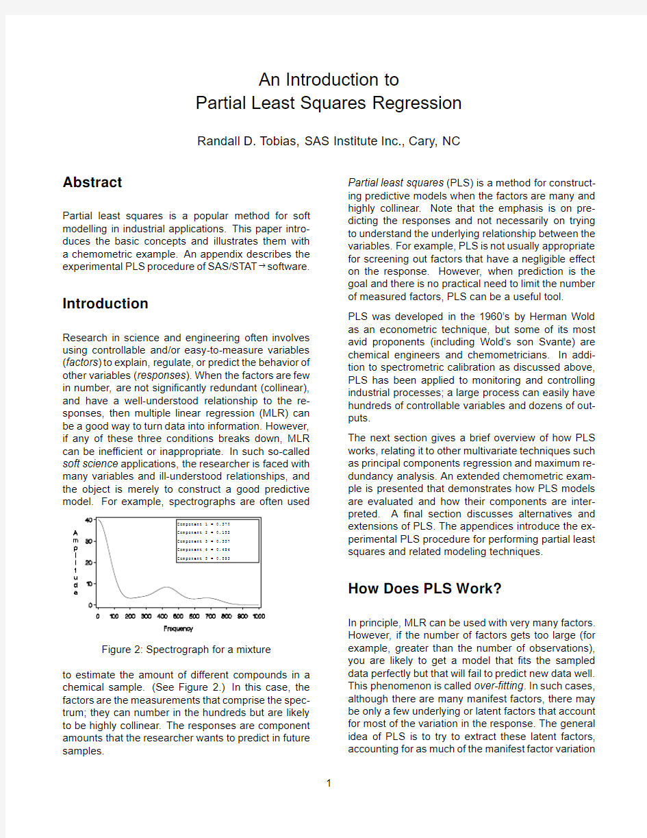
Figure2:Spectrograph for a mixture
to estimate the amount of different compounds in a chemical sample.(See Figure2.)In this case,the factors are the measurements that comprise the spec-trum;they can number in the hundreds but are likely to be highly collinear.The responses are component amounts that the researcher wants to predict in future samples.Partial least squares(PLS)is a method for construct-ing predictive models when the factors are many and highly collinear.Note that the emphasis is on pre-dicting the responses and not necessarily on trying to understand the underlying relationship between the variables.For example,PLS is not usually appropriate for screening out factors that have a negligible effect on the response.However,when prediction is the goal and there is no practical need to limit the number of measured factors,PLS can be a useful tool.
PLS was developed in the1960’s by Herman Wold as an econometric technique,but some of its most avid proponents(including Wold’s son Svante)are chemical engineers and chemometricians.In addi-tion to spectrometric calibration as discussed above, PLS has been applied to monitoring and controlling industrial processes;a large process can easily have hundreds of controllable variables and dozens of out-puts.
The next section gives a brief overview of how PLS works,relating it to other multivariate techniques such as principal components regression and maximum re-dundancy analysis.An extended chemometric exam-ple is presented that demonstrates how PLS models are evaluated and how their components are inter-preted.A final section discusses alternatives and extensions of PLS.The appendices introduce the ex-perimental PLS procedure for performing partial least squares and related modeling techniques.
How Does PLS Work?
In principle,MLR can be used with very many factors. However,if the number of factors gets too large(for example,greater than the number of observations), you are likely to get a model that fits the sampled data perfectly but that will fail to predict new data well. This phenomenon is called over-fitting.In such cases, although there are many manifest factors,there may be only a few underlying or latent factors that account for most of the variation in the response.The general idea of PLS is to try to extract these latent factors, accounting for as much of the manifest factor variation
as possible while modeling the responses well.For this reason,the acronym PLS has also been taken to mean‘‘projection to latent structure.’’It should be noted,however,that the term‘‘latent’’does not have the same technical meaning in the context of PLS as it does for other multivariate techniques.In particular, PLS does not yield consistent estimates of what are called‘‘latent variables’’in formal structural equation modelling(Dykstra1983,1985).
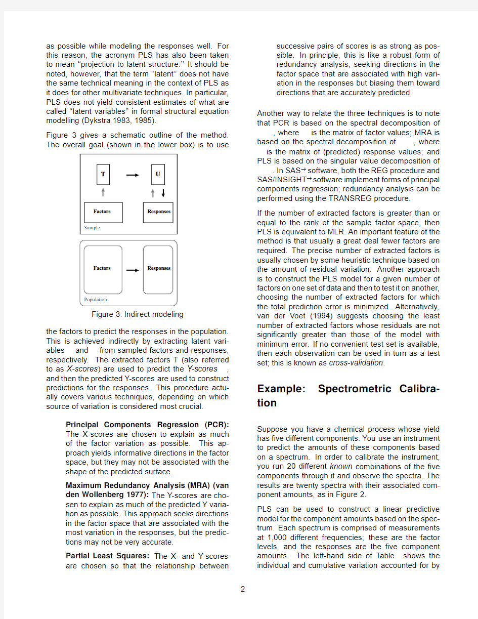
Figure3gives a schematic outline of the method. The overall goal(shown in the lower box)is to use
Figure3:Indirect modeling
the factors to predict the responses in the population. This is achieved indirectly by extracting latent vari-ables and from sampled factors and responses, respectively.The extracted factors T(also referred to as X-scores)are used to predict the Y-scores, and then the predicted Y-scores are used to construct predictions for the responses.This procedure actu-ally covers various techniques,depending on which source of variation is considered most crucial.
Principal Components Regression(PCR):
The X-scores are chosen to explain as much
of the factor variation as possible.This ap-
proach yields informative directions in the factor
space,but they may not be associated with the
shape of the predicted surface.
Maximum Redundancy Analysis(MRA)(van
den Wollenberg1977):The Y-scores are cho-
sen to explain as much of the predicted Y varia-
tion as possible.This approach seeks directions
in the factor space that are associated with the
most variation in the responses,but the predic-
tions may not be very accurate.
Partial Least Squares:The X-and Y-scores
are chosen so that the relationship between
successive pairs of scores is as strong as pos-
sible.In principle,this is like a robust form of
redundancy analysis,seeking directions in the
factor space that are associated with high vari-
ation in the responses but biasing them toward
directions that are accurately predicted. Another way to relate the three techniques is to note that PCR is based on the spectral decomposition of ,where is the matrix of factor values;MRA is
based on the spectral decomposition of,where is the matrix of(predicted)response values;and PLS is based on the singular value decomposition of .In SAS?software,both the REG procedure and SAS/INSIGHT?software implement forms of principal components regression;redundancy analysis can be performed using the TRANSREG procedure.
If the number of extracted factors is greater than or equal to the rank of the sample factor space,then PLS is equivalent to MLR.An important feature of the method is that usually a great deal fewer factors are required.The precise number of extracted factors is usually chosen by some heuristic technique based on the amount of residual variation.Another approach is to construct the PLS model for a given number of factors on one set of data and then to test it on another, choosing the number of extracted factors for which the total prediction error is minimized.Alternatively, van der Voet(1994)suggests choosing the least number of extracted factors whose residuals are not significantly greater than those of the model with minimum error.If no convenient test set is available, then each observation can be used in turn as a test set;this is known as cross-validation.
Example:Spectrometric Calibra-tion
Suppose you have a chemical process whose yield has five different components.You use an instrument to predict the amounts of these components based on a spectrum.In order to calibrate the instrument, you run20different known combinations of the five components through it and observe the spectra.The results are twenty spectra with their associated com-ponent amounts,as in Figure2.
PLS can be used to construct a linear predictive model for the component amounts based on the spec-trum.Each spectrum is comprised of measurements at1,000different frequencies;these are the factor levels,and the responses are the five component amounts.The left-hand side of Table shows the individual and cumulative variation accounted for by
Table2:PLS analysis of spectral calibration,with cross-validation Number of
PLS Responses Comparison Factors Current Total PRESS
39.3539.35
29.9369.28
7.9477.22
6.4083.62
2.0785.69
1.2086.89
1.1588.04
1.1289.16
1.0690.22
1.0291.24
(1993)is a closely related technique.It is exactly the same as PLS when there is only one response and invariably gives very similar results,but it can be dramatically more efficient to compute when there are many factors.Continuum regression(Stone and Brooks1990)adds a continuous parameter,where 01,allowing the modeling method to vary continuously between MLR(0),PLS(05), and PCR(1).De Jong and Kiers(1992)de-scribe a related technique called principal covariates regression.
In any case,PLS has become an established tool in chemometric modeling,primarily because it is often possible to interpret the extracted factors in terms of the underlying physical system---that is,to derive ‘‘hard’’modeling information from the soft model.More work is needed on applying statistical methods to the selection of the model.The idea of van der Voet (1994)for randomization-based model comparison is a promising advance in this direction.
For Further Reading
PLS is still evolving as a statistical modeling tech-nique,and thus there is no standard text yet that gives it in-depth coverage.Geladi and Kowalski(1986)is a standard reference introducing PLS in chemomet-ric applications.For technical details,see Naes and Martens(1985)and de Jong(1993),as well as the references in the latter.
References
Dijkstra,T.(1983),‘‘Some comments on maximum likelihood and partial least squares methods,’’
Journal of Econometrics,22,67-90.
Dijkstra,T.(1985).Latent variables in linear stochas-tic models:Reflections on maximum likelihood
and partial least squares methods.2nd ed.Ams-
terdam,The Netherlands:Sociometric Research
Foundation.
Geladi,P,and Kowalski, B.(1986),‘‘Partial least-squares regression:A tutorial,’’Analytica Chim-
ica Acta,185,1-17.
Frank,I.and Friedman,J.(1993),‘‘A statistical view of some chemometrics regression tools,’’Tech-
nometrics,35,109-135.Haykin,S.(1994).Neural Networks,a Comprehen-sive Foundation.New York:Macmillan. Helland,I.(1988),‘‘On the structure of partial least squares regression,’’Communications in Statis-
tics,Simulation and Computation,17(2),581-
607.
Hoerl,A.and Kennard,R.(1970),‘‘Ridge regression: biased estimation for non-orthogonal problems,’’
Technometrics,12,55-67.
de Jong,S.and Kiers,H.(1992),‘‘Principal covari-ates regression,’’Chemometrics and Intelligent
Laboratory Systems,14,155-164.
de Jong,S.(1993),‘‘SIMPLS:An alternative approach to partial least squares regression,’’Chemomet-
rics and Intelligent Laboratory Systems,18,251-
263.
Naes,T.and Martens,H.(1985),‘‘Comparison of pre-diction methods for multicollinear data,’’Com-
munications in Statistics,Simulation and Com-
putation,14(3),545-576.
Ranner,Lindgren,Geladi,and Wold,‘‘A PLS kernel algorithm for data sets with many variables and
fewer objects,’’Journal of Chemometrics,8,111-
125.
Sarle,W.S.(1994),‘‘Neural Networks and Statis-tical Models,’’Proceedings of the Nineteenth
Annual SAS Users Group International Confer-
ence,Cary,NC:SAS Institute,1538-1550. Stone,M.and Brooks,R.(1990),‘‘Continuum regres-sion:Cross-validated sequentially constructed
prediction embracing ordinary least squares,
partial least squares,and principal components
regression,’’Journal of the Royal Statistical So-
ciety,Series B,52(2),237-269.
van den Wollenberg, A.L.(1977),‘‘Redundancy Analysis--An Alternative to Canonical Correla-
tion Analysis,’’Psychometrika,42,207-219. van der Voet,H.(1994),‘‘Comparing the predictive ac-curacy of models using a simple randomization
test,’’Chemometrics and Intelligent Laboratory
Systems,25,313-323.
SAS,SAS/INSIGHT,and SAS/STAT are registered trademarks of SAS Institute Inc.in the USA and other countries.?indicates USA registration.
Appendix1:PROC PLS:An Exper-imental SAS Procedure for Partial Least Squares
An experimental SAS/STAT software procedure, PROC PLS,is available with Release6.11of the SAS System for performing various factor-extraction methods of modeling,including partial least squares. Other methods currently supported include alternative algorithms for PLS,such as the SIMPLS method of de Jong(1993)and the RLGW method of Rannar et al. (1994),as well as principal components regression. Maximum redundancy analysis will also be included in a future release.Factors can be specified using GLM-type modeling,allowing for polynomial,cross-product, and classification effects.The procedure offers a wide variety of methods for performing cross-validation on the number of factors,with an optional test for the appropriate number of factors.There are output data sets for cross-validation and model information as well as for predicted values and estimated factor scores. You can specify the following statements with the PLS procedure.Items within the brackets are optional.
PROC PLS options;
CLASS class-variables;
MODEL responses=effects/option;
OUTPUT OUT=SAS-data-set options;
PROC PLS Statement
PROC PLS options;
You use the PROC PLS statement to invoke the PLS procedure and optionally to indicate the analysis data and method.The following options are available: DATA=SAS-data-set
specifies the input SAS data set that con-
tains the factor and response values. METHOD=factor-extraction-method
specifies the general factor extraction
method to be used.You can specify any
one of the following:
METHOD=PLS(PLS-options)
specifies partial least squares.This is
the default factor extraction method.
METHOD=SIMPLS
specifies the SIMPLS method of de
Jong(1993).This is a more effi-
cient algorithm than standard PLS;it
is equivalent to standard PLS when
there is only one response,and it
invariably gives very similar results.
METHOD=PCR
specifies principal components re-
gression.
You can specify the following PLS-options in parentheses after METHOD=PLS:
ALGORITHM=PLS-algorithm
gives the specific algorithm used to
compute PLS factors.Available algo-
rithms are
ITER the usual iterative NIPALS al-
gorithm
SVD singular value decomposi-
tion of,the most exact
but least efficient approach EIG eigenvalue decomposition of
RLGW an iterative approach that
is efficient when there are
many factors
MAXITER=number
gives the maximum number of itera-
tions for the ITER and RLGW algo-
rithms.The default is200.
EPSILON=number
gives the convergence criterion for
the ITER and RLGW algorithms.The
default is1012.
CV=cross-validation-method
specifies the cross-validation method to be used.If you do not specify a cross-validation method,the default action is not to perform cross-validation.You can specify any one of the following:
CV=ONE
specifies one-at-a-time cross-valida-
tion
CV=SPLIT(n)
specifies that every th observation
be excluded.You may optionally
specify;the default is1,which is
the same as CV=ONE.
CV=BLOCK(n)
specifies that blocks of th observa-
tions be excluded.You may option-
ally specify;the default is1,which
is the same as CV=ONE.
CV=RANDOM(cv-random-opts)
specifies that random observations
be excluded.
CV=TESTSET(SAS-data-set)
specifies a test set of observations to
be used for cross-validation.
You also can specify the following cv-random-opts in parentheses after CV= RANDOM:
NITER=number
specifies the number of random sub-
sets to exclude.
NTEST=number
specifies the number of observations
in each random subset chosen for
exclusion.
SEED=number
specifies the seed value for random
number generation.
CVTEST(cv-test-options)
specifies that van der Voet’s(1994) randomization-based model comparison test be performed on each cross-validated model.You also can specify the follow-ing cv-test-options in parentheses after CVTEST:
PVAL=number
specifies the cut-off probability for
declaring a significant difference.The
default is0.10.
STAT=test-statistic
specifies the test statistic for the
model comparison.You can specify
either T2,for Hotelling’s2statistic,
or PRESS,for the predicted residual
sum of squares.T2is the default.
NSAMP=number
specifies the number of randomiza-
tions to perform.The default is1000. LV=number
specifies the number of factors to extract.
The default number of factors to extract is the number of input factors,in which case the analysis is equivalent to a regular least squares regression of the responses on the input factors.
OUTMODEL=SAS-data-set
specifies a name for a data set to contain information about the fit model.
OUTCV=SAS-data-set
specifies a name for a data set to contain information about the cross-validation.CLASS Statement
CLASS class-variables;
You use the CLASS statement to identify classifica-tion variables,which are factors that separate the observations into groups.
Class-variables can be either numeric or character. The PLS procedure uses the formatted values of class-variables in forming model effects.Any variable in the model that is not listed in the CLASS statement is assumed to be continuous.Continuous variables must be numeric.
MODEL Statement
MODEL responses=effects/INTERCEPT; You use the MODEL statement to specify the re-sponse variables and the independent effects used to model https://www.doczj.com/doc/a48341188.html,ually you will just list the names of the independent variables as the model effects, but you can also use the effects notation of PROC GLM to specify polynomial effects and interactions. By default the factors are centered and thus no inter-cept is required in the model,but you can specify the INTERCEPT option to override this behavior.
OUTPUT Statement
OUTPUT OUT=SAS-data-set keyword=names keyword=names;
You use the OUTPUT statement to specify a data set to receive quantities that can be computed for every input observation,such as extracted factors and predicted values.The following keywords are available:
PREDICTED predicted values for responses YRESIDUAL residuals for responses XRESIDUAL residuals for factors
XSCORE extracted factors(X-scores,latent
vectors,)
YSCORE extracted responses(Y-scores,) STDY standard error for Y predictions STDX standard error for X predictions
H approximate measure of influence PRESS predicted residual sum of squares T2scaled sum of squares of scores
XQRES sum of squares of scaled residuals
for factors
YQRES sum of squares of scaled residuals
for responses
Appendix2:Example Code
The data for the spectrometric calibration example is in the form of a SAS data set called SPECTRA with 20observations,one for each test combination of the five components.The variables are
X1X1000-the spectrum for this combination Y1Y5-the component amounts
There is also a test data set of20more observations available for cross-validation.The following state-ments use PROC PLS to analyze the data,using the SIMPLS algorithm and selecting the number of factors with cross-validation.
proc pls data=spectra
method=simpls
lv=9
cv=testset(test5)
cvtest(stat=press);
model y1-y5=x1-x1000;
run;
The listing has two parts(Figure5),the first part summarizing the cross-validation and the second part showing how much variation is explained by each ex-tracted factor for both the factors and the responses. Note that the extracted factors are labeled‘‘latent variables’’in the listing.
The PLS Procedure
Cross Validation for the Number of Latent Variables
Test for larger
residuals than
minimum
Number of Root
Latent Mean Prob>
Variables PRESS PRESS
-----------------------------------
0 1.06700
10.92860
20.85100
30.72820
40.60010.00500
50.31230.6140
60.30510.6140
70.30470.3530
80.30550.4270
90.3045 1.0000
100.30610.0700
Minimum Root Mean PRESS=0.304457for9latent variables Smallest model with p-value>0.1:5latent variables
The PLS Procedure
Percent Variation Accounted For
Number of
Latent Model Effects Dependent Variables Variables Current Total Current Total ----------------------------------------------------------139.352639.352628.702228.7022
229.936969.289525.575954.2780
37.933377.222821.863176.1411
4 6.401483.6242 6.450282.5913
5 2.067985.692016.957399.548
6 Figure5:PROC PLS output for spectrometric calibration example
题目: (递推最小二乘法) 考虑如下系统: )()4(5.0)3()2(7.0)1(5.1)(k k u k u k y k y k y ξ+-+-=-+-- 式中,)(k ξ为方差为0.1的白噪声。 取初值I P 610)0(=、00=∧ )(θ。选择方差为1的白噪声作为输入信号)(k u ,采用PLS 法进行参数估计。 Matlab 代码如下: clear all close all L=400; %仿真长度 uk=zeros(4,1); %输入初值:uk(i)表示u(k-i) yk=zeros(2,1); %输出初值 u=randn(L,1); %输入采用白噪声序列 xi=sqrt(0.1)*randn(L,1); %方差为0.1的白噪声序列 theta=[-1.5;0.7;1.0;0.5]; %对象参数真值 thetae_1=zeros(4,1); %()θ初值 P=10^6*eye(4); %题目要求的初值 for k=1:L phi=[-yk;uk(3:4)]; %400×4矩阵phi 第k 行对应的y(k-1),y(k-2),u(k-3), u(k-4) y(k)=phi'*theta+xi(k); %采集输出数据 %递推最小二乘法的递推公式 K=P*phi/(1+phi'*P*phi); thetae(:,k)=thetae_1+K*(y(k)-phi'*thetae_1); P=(eye(4)-K*phi')*P; %更新数据 thetae_1=thetae(:,k); for i=4:-1:2 uk(i)=uk(i-1); end uk(1)=u(k); for i=2:-1:2 yk(i)=yk(i-1);
最小二乘法及其应用 1. 引言 最小二乘法在19世纪初发明后,很快得到欧洲一些国家的天文学家和测地学家的广泛关注。据不完全统计,自1805年至1864年的60年间,有关最小二乘法的研究论文达256篇,一些百科全书包括1837年出版的大不列颠百科全书第7版,亦收入有关方法的介绍。同时,误差的分布是“正态”的,也立刻得到天文学家的关注及大量经验的支持。如贝塞尔( F. W. Bessel, 1784—1846)对几百颗星球作了三组观测,并比较了按照正态规律在给定范围内的理论误差值和实际值,对比表明它们非常接近一致。拉普拉斯在1810年也给出了正态规律的一个新的理论推导并写入其《分析概论》中。正态分布作为一种统计模型,在19世纪极为流行,一些学者甚至把19世纪的数理统计学称为正态分布的统治时代。在其影响下,最小二乘法也脱出测量数据意义之外而发展成为一个包罗极大,应用及其广泛的统计模型。到20世纪正态小样本理论充分发展后,高斯研究成果的影响更加显著。最小二乘法不仅是19世纪最重要的统计方法,而且还可以称为数理统计学之灵魂。相关回归分析、方差分析和线性模型理论等数理统计学的几大分支都以最小二乘法为理论基础。正如美国统计学家斯蒂格勒( S. M. Stigler)所说,“最小二乘法之于数理统计学犹如微积分之于数学”。最小二乘法是参数回归的最基本得方法所以研究最小二乘法原理及其应用对于统计的学习有很重要的意义。 2. 最小二乘法 所谓最小二乘法就是:选择参数10,b b ,使得全部观测的残差平方和最小. 用数学公式表示为: 21022)()(m in i i i i i x b b Y Y Y e --=-=∑∑∑∧ 为了说明这个方法,先解释一下最小二乘原理,以一元线性回归方程为例. i i i x B B Y μ++=10 (一元线性回归方程)
一、 递推最小二乘法 递推最小二乘法的一般步骤: 1. 根据输入输出序列列出最小二乘法估计的观测矩阵?: ] )(u ... )1( )( ... )1([)(T b q n k k u n k y k y k ------=? 没有给出输出序列的还要先算出输出序列。 本例中, 2)]-u(k 1),-u(k 2),-1),-y(k -[-y(k )(T =k ?。 2. 给辨识参数θ和协方差阵P 赋初值。一般取0θ=0或者极小的数,取σσ,20I P =特别大,本例中取σ=100。 3. 按照下式计算增益矩阵G : ) ()1()(1)()1()(k k P k k k P k G T ???-+-= 4. 按照下式计算要辨识的参数θ: )]1(?)()()[()1(?)(?--+-=k k k y k G k k T θ?θθ 5. 按照下式计算新的协方差阵P : )1()()()1()(---=k P k k G k P k P T ? 6. 计算辨识参数的相对变化量,看是否满足停机准则。如满足,则不再递推;如不满足, 则从第三步开始进行下一次地推,直至满足要求为止。 停机准则:ε???<--) (?)1(?)(?max k k k i i i i 本例中由于递推次数只有三十次,故不需要停机准则。 7. 分离参数:将a 1….a na b 1….b nb 从辨识参数θ中分离出来。 8. 画出被辨识参数θ的各次递推估计值图形。 为了说明噪声对递推最小二乘法结果的影响,程序5-7-2在计算模拟观测值时不加噪 声, 辨识结果为a1 =1.6417,a2 = 0.7148,b1 = 0.3900,b2 =0.3499,与真实值a1 =1.642, a2 = 0.715, b1 = 0.3900,b2 =0.35相差无几。 程序5-7-2-1在计算模拟观测值时加入了均值为0,方差为0.1的白噪声序列,由于噪 声的影响,此时的结果为变值,但变化范围较小,现任取一组结果作为辨识结果。辨识结果为a1 =1.5371, a2 = 0.6874, b1 = 0.3756,b2 =0.3378。 程序5-7-2-2在计算模拟观测值时加入了有色噪声,有色噪声为 E(k)+1.642E(k-1)+0.715E(k-2),E(k)是均值为0,方差为0.1的白噪声序列,由于有色噪声的影响,此时的辨识结果变动范围远比白噪声时大,任取一组结果作为辨识结果。辨识结果为a1 =1.6676, a2 = 0.7479, b1 = 0.4254,b2 =0.3965。 可以看出,基本的最小二乘法不适用于有色噪声的场合。
《人工智能》课程论文 论文题目:偏最小二乘算法(PLS)回归建模 学生姓名:张帅帅 学号: 172341392 专业:机械制造及其自动化 所在学院:机械工程学院 年月日
目录 偏最小二乘回归....................................... - 2 -摘要................................................. - 2 -§1偏最小二乘回归原理................................ - 2 -§2一种更简洁的计算方法.............................. - 6 -§3案例分析 ......................................... - 7 -致谢................................................ - 16 -附件:.............................................. - 17 -
偏最小二乘回归 摘要 在实际问题中,经常遇到需要研究两组多重相关变量间的相互依赖关系,并研究用一组变量(常称为自变量或预测变量)去预测另一组变量(常称为因变量或响应变量),除了最小二乘准则下的经典多元线性回归分析(MLR ),提取自变量组主成分的主成分回归分析(PCR )等方法外,还有近年发展起来的偏最小二乘(PLS )回归方法。 偏最小二乘回归提供一种多对多线性回归建模的方法,特别当两组变量的个数很多,且都存在多重相关性,而观测数据的数量(样本量)又较少时,用偏最小二乘回归建立的模型具有传统的经典回归分析等方法所没有的优点。 偏最小二乘回归分析在建模过程中集中了主成分分析,典型相关分析和线性回归分析方法的特点,因此在分析结果中,除了可以提供一个更为合理的回归模型外,还可以同时完成一些类似于主成分分析和典型相关分析的研究内容,提供更丰富、深入的一些信息。 本文介绍偏最小二乘回归分析的建模方法;通过例子从预测角度对所建立的回归模型进行比较。 关键词:主元分析、主元回归、回归建模 1 偏最小二乘回归原理 考虑p 个变量p y y y ,...,21与m 个自变量m x x x ,...,21 的建模问题。偏最小二乘回归的基本作法是首先在自变量集中提出第一成分t ?(t ?是 m x x x ,...,21 的线性组合,且尽可能多地提取原自变量集中的变异信息);同时在因变量集中也提取第一成分u ?,并要求t ?与u ?相关程度达到最大。然后建立因变量 p y y y , (21) t ?的回归,如果回归方程已达到满意的精度,则算法中止。否则 继续第二对成分的提取,直到能达到满意的精度为止。若最终对自变量集提取r 个成分r t t t ,...,21,偏最小二乘回归将通过建立 p y y y ,...,21与r t t t ,...,21的回归 式,然后再表示为p y y y ,...,21与原自变量的回归方程式,即偏最小二乘回归方程式。 为了方便起见,不妨假定p 个因变量p y y y ,...,21与m 个自变量m x x x ,...,21均为
最小二乘法原理 1. 概念 最小二乘法多项式曲线拟合,根据给定的m 个点,并不要求这条曲线精确地经过这些点,而是曲线y=f(x)的近似曲线y= φ(x)。 2. 原理 给定数据点pi(xi,yi),其中i=1,2,…,m 。求近似曲线y= φ(x)。并且使得近似曲线与y=f(x)的偏差最小。近似曲线在点pi 处的偏差δi= φ(xi)-yi ,i=1,2,...,m 。 常见的曲线拟合方法: 1. 是偏差绝对值最小 11min (x )y m m i i i i i φδφ===-∑∑ 2. 是最大的偏差绝对值最小 min max (x )y i i i i φδ?=- 3. 是偏差平方和最小 2211min ((x )y )m m i i i i i φδ?===-∑∑ 按偏差平方和最小的原则选取拟合曲线,并且采取二项式方程为拟合曲线的方法,称为最小二乘法。 推导过程: 1. 设拟合多项式为: 01...k k y a a x a x =+++ 2. 各点到这条曲线的距离之和,即偏差平方和如下: 2 2 011(...)m k i i k i i R y a a x a x =??=-+++??∑ 3. 为了求得符合条件的a 值,对等式右边求ak 偏导数,因而我们得到了: 011 2(...)0m k i k i i y a a x a x =??--+++=??∑ 011 2(...)0m k i k i i y a a x a x x =??--+++=??∑
…….. 0112( 0 k k i k i i y a a x a x x =??--+++=??∑ 4. 将等式简化一下,得到下面的式子 01111...n n n k i k i i i i i a n a x a x y ===+++=∑∑∑ 2 1011111...n n n n k i i k i i i i i i i a x a x a x y x +====+++=∑∑∑∑ …… 12011111...n n n n k k k k i i k i i i i i i i a x a x a x y x +====+++=∑∑∑∑ 5. 把这些等式表示成矩阵形式,就可以得到下面的矩阵: 11102111111121111.........n n n k i i i i i i n n n n k i i i i i i i i i n n n n k k k k k i i i i i i i i i n x x y a a x x x x y a x x x x y ===+====+====??????????????????????=?????????????????????? ∑∑∑∑∑∑∑∑∑∑∑ 6. 将这个范德蒙矩阵化简后得到: 0111122 21...1...1...k k k k n n n a y x x a y x x a y x x ??????????????????=????????????????????
普通最小二乘法(OLS ) 普通最小二乘法(Ordinary Least Square ,简称OLS ),是应用最多的参数估计方法,也是从最小二乘原理出发的其他估计方法的基础,是必须熟练掌握的一种方法。 在已经获得样本观测值i i x y ,(i=1,2,…,n )的情况下 (见图中的散点),假如模型()的参数估计量已经求得到, 为^0β和^ 1β,并且是最合理的参数估计量,那么直线方程(见 图中的直线) i i x y ^ 1^0^ββ+= i=1,2,…,n 应该能够最 好地拟合样本数据。其中^i y 为被解释变量的估计值,它是由参数估计量和解释变量的观测值计算得到的。那么,被解释变量的估计值与观测值应该在总体上最为接近,判断的标准是二者之差的平方和最小。 ),()(1022101ββββQ u x y Q i i n i i ==--=∑∑= ()()),(min ????1021 10212?,?1100ββββββββQ x y y y u Q n i i n i i i =--=-==∑∑∑== 为什么用平方和因为二者之差可正可负,简单求和可能将很大的误差抵消掉,只有平方和才能反映二者在总体上的接近程度。这就是最小二乘原则。那么,就可以从最小二乘原则和样本观测值出发,求得参数估计量。 由于 2 1 ^1^012 ^ ))(()(∑∑+--=n i i n i i x y y y Q ββ= 是^0β、^1β的二次函数并且非负,所以其极小值总是存在的。根据罗彼塔法则,当Q 对^0β、^ 1β的一阶偏导数为0时,Q 达到最小。即
0011001100?,?1 ?,?0 =??=??====ββββββββββQ Q 容易推得特征方程: ()0)??(0?)??(1011 10==--==-=--∑∑∑∑∑==i i i i n i i i i i i n i i e x x y x e y y x y ββββ 解得: ∑∑∑∑∑+=+=2^ 1^0^1^0i i i i i i x x x y x n y ββββ () 所以有:???? ?????-=---=--=∑∑∑∑∑∑∑=======x y x x y y x x x x n y x y x n n i i n i i i n i i n i i n i i n i i n i i i 10121 21121111??)())(()()()(?βββ () 于是得到了符合最小二乘原则的参数估计量。 为减少计算工作量,许多教科书介绍了采用样本值的离差形式的参数估计量的计算公式。由于现在计量经济学计算机软件被普遍采用,计算工作量已经不是什么问题。但离差形式的计算公式在其他方面也有应用,故在此写出有关公式,不作详细说明。记 ∑=-i x n x 1 ∑=-i y n y 1 y y y x x x i i i i -=-= ()的参数估计量可以写成
第6章曲线拟合的最小二乘法 6.1 拟合曲线 通过观察或测量得到一组离散数据序列,当所得数据比较准确时,可构造插值函数逼近客观存在的函数,构造的原则是要求插值函数通过这些数据点,即。此时,序列与 是相等的。 如果数据序列,含有不可避免的误差(或称“噪音”),如图6.1 所示;如果数据序列无法同时满足某特定函数,如图6.2所示,那么,只能要求所做逼近函数最优地靠近样点,即向量与的误差或距离最小。按与之间误差最小原则作为“最优”标准构造的逼近函数,称为拟合函数。 图6.1 含有“噪声”的数据 图6.2 一条直线公路与多个景点 插值和拟合是构造逼近函数的两种方法。插值的目标是要插值函数尽量靠近离散点;拟合的目标是要离散点尽量靠近拟合函数。 向量与之间的误差或距离有各种不同的定义方法。例如: 用各点误差绝对值的和表示: 用各点误差按模的最大值表示: 用各点误差的平方和表示: 或(6.1)
其中称为均方误差,由于计算均方误差的最小值的方法容易实现而被广泛采用。按 均方误差达到极小构造拟合曲线的方法称为最小二乘法。本章主要讲述用最小二乘法构造拟合曲线的方法。 在运筹学、统计学、逼近论和控制论中,最小二乘法都是很重要的求解方法。例如,它是统计学中估计回归参数的最基本方法。 关于最小二乘法的发明权,在数学史的研究中尚未定论。有材料表明高斯和勒让德分别独立地提出这种方法。勒让德是在1805年第一次公开发表关于最小二乘法的论文,这时高斯指出,他早在1795年之前就使用了这种方法。但数学史研究者只找到了高斯约在1803年之前使用了这种方法的证据。 在实际问题中,怎样由测量的数据设计和确定“最贴近”的拟合曲线?关键在选择适当的拟合曲线类型,有时根据专业知识和工作经验即可确定拟合曲线类型;在对拟合曲线一无所知的情况下,不妨先绘制数据的粗略图形,或许从中观测出拟合曲线的类型;更一般地,对数据进行多种曲线类型的拟合,并计算均方误差,用数学实验的方法找出在最小二乘法意义下的误差最小的拟合函数。 例如,某风景区要在已有的景点之间修一条规格较高的主干路,景点与主干路之间由各具特色的支路联接。设景点的坐标为点列;设主干路为一条直线 ,即拟合函数是一条直线。通过计算均方误差最小值而确定直线方程(见图6.2)。 6.2线性拟合和二次拟合函数 线性拟合 给定一组数据,做拟合直线,均方误差为 (6.2) 是二元函数,的极小值要满足 整理得到拟合曲线满足的方程:
偏最小二乘法的Matlab源码(2008-09-21 09:31:21) 标签:杂谈 所谓偏最小二乘法,就是指在做基于最小二乘法的线性回归分析之前,对数据集进行主成分分析降维,下面的源码是没有删减的,GreenSim团队免费提供您使用,转载请注明GreenSim团队(https://www.doczj.com/doc/a48341188.html,/greensim)。 function [y5,e1,e2]=PLS(X,Y,x,y,p,q) %% 偏最小二乘回归的通用程序 % 注释以“基于近红外光谱分析的汽油组分建模”为例,但本程序的适用范围绝不仅限于此 % GreenSim团队原创作品(https://www.doczj.com/doc/a48341188.html,/greensim) %% 输入参数列表 % X 校正集光谱矩阵,n×k的矩阵,n个样本,k个波长 % Y 校正集浓度矩阵,n×m的矩阵,n个样本,m个组分 % x 验证集光谱矩阵 % y 验证集浓度矩阵 % p X的主成分的个数,最佳取值需由其它方法确定 % q Y的主成分的个数,最佳取值需由其它方法确定 %% 输出参数列表 % y5 x对应的预测值(y为真实值) % e1 预测绝对误差,定义为e1=y5-y % e2 预测相对误差,定义为e2=|(y5-y)/y| %% 第一步:对X,x,Y,y进行归一化处理
[n,k]=size(X); m=size(Y,2); Xx=[X;x]; Yy=[Y;y]; xmin=zeros(1,k); xmax=zeros(1,k); for j=1:k xmin(j)=min(Xx(:,j)); xmax(j)=max(Xx(:,j)); Xx(:,j)=(Xx(:,j)-xmin(j))/(xmax(j)-xmin(j)); end ymin=zeros(1,m); ymax=zeros(1,m); for j=1:m ymin(j)=min(Yy(:,j)); ymax(j)=max(Yy(:,j)); Yy(:,j)=(Yy(:,j)-ymin(j))/(ymax(j)-ymin(j)); end X1=Xx(1:n,:); x1=Xx((n+1):end,:); Y1=Yy(1:n,:); y1=Yy((n+1):end,:);
最小二乘法的原理及其应用 一、研究背景 在科学研究中,为了揭示某些相关量之间的关系,找出其规律,往往需要做数据拟合,其常用方法一般有传统的插值法、最佳一致逼近多项式、最佳平方逼近、最小二乘拟合、三角函数逼近、帕德(Pade)逼近等,以及现代的神经网络逼近、模糊逼近、支持向量机函数逼近、小波理论等。 其中,最小二乘法是一种最基本、最重要的计算技巧与方法。它在建模中有着广泛的应用,用这一理论解决讨论问题简明、清晰,特别在大量数据分析的研究中具有十分重要的作用和地位。随着最小二乘理论不断的完善,其基本理论与应用已经成为一个不容忽视的研究课题。本文着重讨论最小二乘法在化学生产以及系统识别中的应用。 二、最小二乘法的原理 人们对由某一变量t或多个变量t1…..tn 构成的相关变量y感兴趣。如弹簧的形变与所用的力相关,一个企业的盈利与其营业额,投资收益和原始资本有关。为了得到这些变量同y之间的关系,便用不相关变量去构建y,使用如下函数模型 , q个相关变量或p个附加的相关变量去拟和。 通常人们将一个可能的、对不相关变量t的构成都无困难的函数类型充作函数模型(如抛物线函数或指数函数)。参数x是为了使所选择的函数模型同观测值y相匹配。(如在测量弹簧形变时,必须将所用的力与弹簧的膨胀系数联系起来)。其目标是合适地选择参数,使函数模型最好的拟合观测值。一般情况下,观测值远多于所选择的参数。 其次的问题是怎样判断不同拟合的质量。高斯和勒让德的方法是,假设测量误差的平均值为0。令每一个测量误差对应一个变量并与其它测量误差不相关(随机无关)。人们假设,在测量误差中绝对不含系统误差,它们应该是纯偶然误差,围绕真值波动。除此之外,测量误差符合正态分布,这保证了偏差值在最后的结果y上忽略不计。 确定拟合的标准应该被重视,并小心选择,较大误差的测量值应被赋予较小的权。并建立如下规则:被选择的参数,应该使算出的函数曲线与观测值之差的平方和最小。用函数表示为:
第一节 最小二乘法的基本原理和多项式拟合 一 最小二乘法的基本原理 从整体上考虑近似函数)(x p 同所给数据点),(i i y x (i=0,1,…,m)误差 i i i y x p r -=)((i=0,1,…,m) 的大小,常用的方法有以下三种:一是误差 i i i y x p r -=)((i=0,1,…,m)绝对值的最大值i m i r ≤≤0max ,即误差 向量 T m r r r r ),,(10 =的∞—范数;二是误差绝对值的和∑=m i i r 0 ,即误差向量r 的1— 范数;三是误差平方和∑=m i i r 02 的算术平方根,即误差向量r 的2—范数;前两种方法简单、自然,但不便于微分运算 ,后一种方法相当于考虑 2—范数的平方,因此在曲线拟合中常采用误差平方和∑=m i i r 02 来 度量误差i r (i=0,1,…,m)的整 体大小。 数据拟合的具体作法是:对给定数据 ),(i i y x (i=0,1,…,m),在取定的函数类Φ中,求Φ∈)(x p ,使误差i i i y x p r -=)((i=0,1,…,m)的平方和最小,即 ∑=m i i r 0 2 =[]∑==-m i i i y x p 0 2 min )( 从几何意义上讲,就是寻求与给定点),(i i y x (i=0,1,…,m)的距离平方和为最 小的曲线)(x p y =(图6-1)。函数)(x p 称为拟合 函数或最小二乘解,求拟合函数)(x p 的方法称为曲线拟合的最小二乘法。 在曲线拟合中,函数类Φ可有不同的选取方法. 6—1 二 多项式拟合 假设给定数据点),(i i y x (i=0,1,…,m),Φ为所有次数不超过)(m n n ≤的多项式构成的函数类,现求一 Φ ∈=∑=n k k k n x a x p 0 )(,使得 [] min )(0 02 02 =??? ??-=-=∑∑∑===m i m i n k i k i k i i n y x a y x p I (1) 当拟合函数为多项式时,称为多项式拟合,满足式(1)的)(x p n 称为最小二乘 拟合多项式。特别地,当n=1时,称为线性拟合或直线拟合。
偏最小二乘法 1.1 基本原理 偏最小二乘法(PLS )是基于因子分析的多变量校正方法,其数学基础为主成分分析。但它相对于主成分回归(PCR )更进了一步,两者的区别在于PLS 法将浓度矩阵Y 和相应的量测响应矩阵X 同时进行主成分分解: X=TP+E Y=UQ+F 式中T 和U 分别为X 和Y 的得分矩阵,而P 和Q 分别为X 和Y 的载荷矩阵,E 和F 分别为运用偏最小二乘法去拟合矩阵X 和Y 时所引进的误差。 偏最小二乘法和主成分回归很相似,其差别在于用于描述变量Y 中因子的同时也用于描述变量X 。为了实现这一点,数学中是以矩阵Y 的列去计算矩阵X 的因子。同时,矩阵Y 的因子则由矩阵X 的列去预测。分解得到的T 和U 矩阵分别是除去了大部分测量误差的响应和浓度的信息。偏最小二乘法就是利用各列向量相互正交的特征响应矩阵T 和特征浓度矩阵U 进行回归: U=TB 得到回归系数矩阵,又称关联矩阵B : B=(T T T -1)T T U 因此,偏最小二乘法的校正步骤包括对矩阵Y 和矩阵X 的主成分分解以及对关联矩阵B 的计算。 1.2主成分分析 主成分分析的中心目的是将数据降维,以排除众多化学信息共存中相互重叠的信息。他是将原变量进行转换,即把原变量的线性组合成几个新变量。同时这些新变量要尽可能多的表征原变量的数据结构特征而不丢失信息。新变量是一组正交的,即互不相关的变量。这种新变量又称为主成分。 如何寻找主成分,在数学上讲,求数据矩阵的主成分就是求解该矩阵的特征值和特征矢量问题。下面以多组分混合物的量测光谱来加以说明。假设有n 个样本包含p 个组分,在m 个波长下测定其光谱数据,根据比尔定律和加和定理有: A n×m =C n×p B p×m 如果混合物只有一种组分,则该光谱矢量与纯光谱矢量应该是方向一致,而大小不同。换句话说,光谱A 表示在由p 个波长构成的p 维变量空间的一组点(n 个),而这一组点一定在一条通过坐标原点的直线上。这条直线其实就是纯光谱b 。因此由m 个波长描述的原始数据可以用一条直线,即一个新坐标或新变量来表示。如果一个混合物由2个组分组成,各组分的纯光谱用b1,b2表示,则有: 1122 T T T i i i a c b c b =+ 有上式看出,不管混合物如何变化,其光谱总可以用两个新坐标轴b1,b2来表示。因此可以 推出,如果混合物由p 个组分组成,那么混合物的光谱就可由p 个主成分轴的线性组合表示。
毕业论文文献综述 信息与计算科学 最小二乘法的原理及应用 一、国内外状况 国际统计学会第56届大会于2007年8月22-29日在美丽的大西洋海滨城市、葡萄牙首都里斯本如期召开。应大会组委会的邀请,以会长李德水为团长的中国统计学会代表团一行29人注册参加了这次大会。北京市统计学会、山东省统计学会,分别组团参加了这次大会。中国统计界(不含港澳台地区)共有58名代表参加了这次盛会。本届大会的特邀论文会议共涉及94个主题,每个主题一般至少有3-5位代表做学术演讲和讨论。通过对大会论文按研究内容进行归纳,特邀论文大致可以分为四类:即数理统计,经济、社会统计和官方统计,统计教育和统计应用。 数理统计方面。数理统计作为统计科学的一个重要部分,特别是随机过程和回归分析依然展现着古老理论的活力,一直受到统计界的重视并吸引着众多的研究者。本届大会也不例外。 二、进展情况 数理统计学19世纪的数理统计学史, 就是最小二乘法向各个应用领域拓展的历史席卷了统计大部分应用的几个分支——相关回归分析, 方差分析和线性模型理论等, 其灵魂都在于最小二乘法; 不少近代的统计学研究是在此法的基础上衍生出来, 作为其进一步发展或纠正其不足之处而采取的对策, 这包括回归分析中一系列修正最小二乘法而导致的估计方法。 数理统计学的发展大致可分 3 个时期。① 20 世纪以前。这个时期又可分成两段,大致上可以把高斯和勒让德关于最小二乘法用于观测数据的误差分析的工作作为分界线,前段属萌芽时期,基本上没有超出描述性统计量的范围。后一阶段可算作是数理统计学的幼年阶段。首先,强调了推断的地位,而摆脱了单纯描述的性质。由于高斯等的工作揭示了最小二乘法的重要性,学者们普遍认为,在实际问题中遇见的几乎所有的连续变量,都可以满意地用最小二乘法来刻画。这种观点使关于最小二乘法得到了深入的发展,②20世纪初到第二次世界大战结束。这是数理统计学蓬勃发展达到成熟的时期。许多重要的基本观点和方法,以及数理统计学的主要分支学科,都是在这个时期建立和发展起来的。这个时期的成就,包含了至今仍在广泛使用的大多数统计方法。在其发展中,以英国统计学家、生物学家费希尔为代表的英国学派起了主导作用。③战后时期。这一时期中,数理统计学在应用和理论两方面继续获得很大的进展。
偏最小二乘法(PLS)简介 偏最小二乘法(PLS )简介 偏最小二乘法(PLS )简介 简介 偏最小二乘法是一种新型的多元统计数据分析方法,它于1983年由伍德(S.Wold)和阿巴诺(C.Albano)等人首次提出。近几十年来,它在理论、方法和应用方面都得到了迅速的发展。 偏最小二乘法 长期以来,模型式的方法和认识性的方法之间的界限分得十分清楚。而偏最小二乘法则把它们有机的结合起来了,在一个算法下,可以同时实现回归建模(多元线性回归)、数据结构简化(主成分分析)以及两组变量之间的相关性分析(典型相关分析)。这是多元统计数据分析中 的一个飞跃。 偏最小二乘法在统计应用中的重要性体现在以下几个方面: 偏最小二乘法是一种多因变量对多自变量的回归建模方法。偏最小二乘法可以较好的解决许多以往用 普通多元回归无法解决的问题。 偏最小二乘法之所以被称为第二代回归方法,还由于它可以实现多种数据分析方法的综合应用。 主成分回归的主要目的是要提取隐藏在矩阵X 中的相关信息,然后用于预测变量Y 的值。 这种做法可以保证让我们只使用那些独立变量,噪音将被消除,从而达到改善预测模型质量的目的。但是,主成分回归仍然有一定的缺陷,当一些有用变量的相关性很小时,我们在选取主成分时就很容易把它们漏掉,使得最终的预测模型可靠性下降,如果我们对每一个成分 进行挑选,那样又太困难了。 偏最小二乘回归可以解决这个问题。它采用对变量X 和Y 都进行分解的方法,从变量X 和Y 中同时提取成分(通常称为因子),再将因子按照它们之间的相关性从大到小排列。现在,我们要建立一个模型,我们只要决定选择几个因子参与建模就可以了 基本概念 偏最小二乘回归是对多元线性回归模型的一种扩展,在其最简单的形式中,只用一个线性模 型来描述独立变量Y 与预测变量组X 之间的关系: 偏最小二乘法(PLS) 简介
LDA 算法入门 一.LDA 算法概述: 线性判别式分析(Linear Discriminant Analysis , LDA),也叫做Fisher 线性判别(Fisher Linear Discriminant ,FLD),是模式识别的经典算法,它是在1996年由Belhumeur 引入模式识别和人工智能领域的。线性鉴别分析的基本思想是将高维的模式样本投影到最佳鉴别矢量空间,以达到抽取分类信息和压缩特征空间维数的效果,投影后保证模式样本在新的子空间有最大的类间距离和最小的类内距离,即模式在该空间中有最佳的可分离性。因此,它是一种有效的特征抽取方法。使用这种方法能够使投影后模式样本的类间散布矩阵最大,并且同时类内散布矩阵最小。就是说,它能够保证投影后模式样本在新的空间中有最小的类内距离和最大的类间距离,即模式在该空间中有最佳的可分离性。 二. LDA 假设以及符号说明: 假设对于一个n R 空间有m 个样本分别为12,,m x x x ,即每个x 是一个n 行的矩阵,其中 i n 表示属第 i 类的样本个数,假设一共有 c 个类,则 12i c n n n n m ++++= 。 b S : 类间离散度矩阵 w S :类内离散度矩阵 i n :属于i 类的样本个数 i x :第i 个样本 u :所有样本的均值 i u :类i 的样本均值 三. 公式推导,算法形式化描述 根据符号说明可得类i 的样本均值为: 1 i x classi i u x n ∈= ∑ (1.1)
同理我们也可以得到总体样本均值: 1 1m i i u x m ==∑ (1.2) 根据类间离散度矩阵和类内离散度矩阵定义,可以得到如下式子: ()() 1c T b i i i i S n u u u u ==--∑ (1.3) ()() 1k c T w i k i k i x classi S u x u x =∈=--∑ ∑ (1.4) 当然还有另一种类间类内的离散度矩阵表达方式: ()()() 1 c T b i i i S P i u u u u ==--∑ (1.5) ()()()(){ } 11 (i)(i)E |k c T w i k i k i x classi i c T i i i P S u x u x n P u x u x x classi =∈==--=--∈∑ ∑∑ (1.6) 其中()P i 是指i 类样本的先验概率,即样本中属于i 类的概率()i n P i m =,把 ()P i 代入第二组式子中,我们可以发现第一组式子只是比第二组式子都少乘了1m ,我们将在稍后进行讨论,其实对于乘不乘该1m ,对于算法本身并没有影响,现在我们分析一下算法的思想, 我们可以知道矩阵 ()() T i i u u u u --的实际意义是一个协方差矩阵,这个矩阵 所刻画的是该类与样本总体之间的关系,其中该矩阵对角线上的函数所代表的是该类相对样本总体的方差(即分散度),而非对角线上的元素所代表是该类样本总体均值的协方差(即该类和总体样本的相关联度或称冗余度),所以根据公式(1.3)可知(1.3)式即把所有样本中各个样本根据自己所属的类计算出样本与总体的协方差矩阵的总和,这从宏观上描述了所有类和总体之间的离散冗余程度。同理可以的得出(1.4)式中为分类内各个样本和所属类之间的协方差矩阵之和,它所刻画的是从总体来看类内各个样本与类之间(这里所刻画的类特性是由是类
曲线拟合——最小二乘法算法 一、目的和要求 1)了解最小二乘法的基本原理,熟悉最小二乘算法; 2)掌握最小二乘进行曲线拟合的编程,通过程序解决实际问题。 二、实习内容 1)最小二乘进行多项式拟合的编程实现。 2)用完成的程序解决实际问题。 三、算法 1)输入数据节点数n ,拟合的多项式次数m ,循环输入各节点的数据x j , y j (j=0,1,…,n-1) 2)由x j 求S ;由x j ,y j 求T : S k = ∑-=10n j k j x ( k=0,1,2, … 2*m ) T k = ∑-=1 0n j k j j x y ( k=0,1,2,… m ) 3)由S 形成系数矩阵数组c i,j :c[i][j]=S[i+j] (i=0,1,2,…m, j=0,1,2,…,m);由T 形成系数矩阵增广部分c i,m+1:c[i][m+1]=T[i] (i=0,1,2,…m) 4)对线性方程组CA=T[或A C ],用列主元高斯消去法求解系数矩阵A=(a 0,a 1,…,a m )T 四、实验步骤 1)完成最小二乘法进行曲线拟合的程序设计及录入、编辑; 2)完成程序的编译和链接,并进行修改; 3)用书上P105例2的例子对程序进行验证,并进行修改; 4)用完成的程序求解下面的实际问题。 5)完成实验报告。 五、实验结果 1. 经编译、链接及例子验证结果正确的源程序: #include
最小二乘法 最小二乘法是一种在误差估计、不确定度、系统辨识及预测、预报等数据处理诸多学科领域得到广泛应用的数学工具。最小二乘法还可用于曲线拟合,其他一些优化问题也可通过最小化能量或最大化熵用最小二乘法来表达。最小二乘法公式: 设拟合直线的公式为 , 其中:拟合直线的斜率为: ;计算出斜率后,根据 和已经确定的斜率k,利用待定系数法求出截距b。
在我们研究两个变量(x, y)之间的相互关系时,通常可以得到一系列成对的数据(x1, y1),(x2, y2).. (xm , ym);将这些数据描绘在x -y 直角坐标系中(如图1), 若发现这些点在一条直线附近,可以令这条直线方程如(式1-1)。 Y计= a0 + a1 X (式1-1) 其中:a0、a1 是任意实数 为建立这直线方程就要确定a0和a1,应用《最小二乘法原理》,将实测值Yi与利用(式1-1)计算值(Y计=a0+a1X)的离差(Yi-Y计)的平方和〔∑(Yi - Y计)²〕最小为“优化判据”。 令: φ= ∑(Yi - Y计)² (式1-2) 把(式1-1)代入(式1-2)中得: φ= ∑(Yi - a0 - a1 Xi)2 (式1-3) 当∑(Yi-Y计)²最小时,可用函数φ对a0、a1求偏导数,令这两个偏导数等于零。 (式1-4) (式1-5) 亦即 m a0 + (∑Xi ) a1 = ∑Yi (式1-6)
(∑Xi ) a0 + (∑Xi2 ) a1 = ∑(Xi, Yi) (式1-7) 得到的两个关于a0、a1为未知数的两个方程组,解这两个方程组得出: a0 = (∑Yi) / m - a1(∑Xi) / m (式1-8) a1 = [∑Xi Yi - (∑Xi ∑Yi)/ m] / [∑Xi2 - (∑Xi)2 / m)] (式1-9) 这时把a0、a1代入(式1-1)中, 此时的(式1-1)就是我们回归的元线性方程即:数学模型。 在回归过程中,回归的关联式是不可能全部通过每个回归数据点(x1, y1、x2, y2...xm,ym),为了判断关联式的好坏,可借助相关系数“R”,统计量“F”,剩余标准偏差“S”进行判断;“R”越趋近于1 越好;“F”的绝对值越大越好;“S”越趋近于0 越好。 R = [∑XiYi - m (∑Xi / m)(∑Yi / m)]/ SQR{[∑Xi2 - m (∑Xi / m)2][∑Yi2 - m (∑Yi / m)2]} (式1-10) * 在(式1-1)中,m为样本容量,即实验次数;Xi、Yi分别任意一组实验X、Y的数值。微积分应用课题一最小二乘法 从前面的学习中, 我们知道最小二乘法可以用来处理一组数据, 可以从一组测定的数据中寻求变量之间的依赖关系, 这种函数关系称为经验公式. 本课题将介绍最小二乘法的精确定义及如何寻求与之间近似成线性关系时的经验公式. 假定实验测得变量之间的个数
一、起源与发展 偏最小二乘法(partial least squares method,PLS)是一种新型的多元统计数据分析方法,它于1983年由伍德(S.Wold)和阿巴诺(C.Albano)等人首次提出。其实在早在70年代伍德(S.Wold)的父亲H Wold便在经济学研究中引入了偏最小二乘法进行路径分析,创建了非线性迭代偏最小二乘算法(Nonlinear Iterative Partial Least Squares algorithm,NIPALS),至今仍然是PLS中最常用和核心的算法。PLS在20世纪90年代引入中国,在经济学、机械控制技术、药物设计及计量化学等方面有所应用,但是在生物医学上偏最小二乘法涉及相对较少。对该方法的各种算法和在实际应用中的介绍也不系统,国内已有学者在这方面做了一些努力,但作为一种新兴的多元统计方法,还不为人所熟知。 PLS是一种数学优化技术,它通过最小化误差的平方和找到一组数据的最佳函数匹配。用最简的方法求得一些绝对不可知的真值,而令误差平方之和为最小。通常用于曲线拟合。有人用下式来形容PLS: 偏最小二乘回归≈多元线性回归分析+典型相关分析+主成分分析 二、特点: 与传统多元线性回归模型相比,偏最小二乘回归的特点是: (1) 能够在自变量存在严重多重相关性的条件下进行回归建模; (2) 允许在样本点个数少于变量个数的条件下进行回归建模; (3) 偏最小二乘回归在最终模型中将包含原有的所有自变量; (4) 偏最小二乘回归模型更易于辨识系统信息与噪声(甚至一些非随机性的噪声); (5) 在偏最小二乘回归模型中,每一个自变量的回归系数将更容易解释。 偏最小二乘法的Matlab源码(2008-09-21 09:31:21) 所谓偏最小二乘法,就是指在做基于最小二乘法的线性回归分析之前,对数据集进行主成分分析降维,下面的源码是没有删减的 https://www.doczj.com/doc/a48341188.html,/greensim)。 function [y5,e1,e2]=PLS(X,Y,x,y,p,q) %% 偏最小二乘回归的通用程序% 注释以“基于近红外光谱分析的汽油组分建模”为例,但本程序的适用范围绝不仅限于此% % 输入参数列表 % X 校正集光谱矩阵,n×k的矩阵,n个样本,k个波长 % Y 校正集浓度矩阵,n×m的矩阵,n个样本,m个组分 % x 验证集光谱矩阵 % y 验证集浓度矩阵 % p X的主成分的个数,最佳取值需由其它方法确定 % q Y的主成分的个数,最佳取值需由其它方法确定% % 输出参数列表 % y5 x对应的预测值(y为真实值) % e1 预测绝对误差,定义为e1=y5-y % e2 预测相对误差,定义为e2=|(y5-y)/y| %% 第一步:对X,x,Y,y进行归一化处理 [n,k]=size(X); m=size(Y,2); Xx=[X;x];
生活中的计算方法应用实例——— 最小二乘法,用MATLAB实现1. 数值实例 下面给定的是某市最近1个月早晨7:00左右(新疆时间)的天气预报所得到的温度 天数 1 2 3 4 5 6 7 8 9 10 温度9 10 11 12 13 14 13 12 11 9 天数11 12 13 14 15 16 17 18 19 20 温度10 11 12 13 14 12 11 10 9 8 天数21 22 23 24 25 26 27 28 29 30 温度7 8 9 11 9 7 6 5 3 1 下面用MATLAB编程对上述数据进行最小二乘拟合,按照数据找出任意次曲线拟合方程和它的图像。 2、程序代码 x=[1:1:30]; y=[9,10,11,12,13,14,13,12,11,9,10,11,12,13,14,12,11,10,9,8,7,8,9,11,9,7, 6,5,3,1]; a1=polyfit(x,y,3) %三次多项式拟合% a2= polyfit(x,y,9) %九次多项式拟合% a3= polyfit(x,y,15) %十五次多项式拟合% b1= polyval(a1,x) b2= polyval(a2,x) b3= polyval(a3,x) r1= sum((y-b1).^2) %三次多项式误差平方和% r2= sum((y-b2).^2) %九次次多项式误差平方和% r3= sum((y-b3).^2) %十五次多项式误差平方和% plot(x,y,'*') %用*画出x,y图像% hold on plot(x,b1, 'r') %用红色线画出x,b1图像% hold on plot(x,b2, 'g') %用绿色线画出x,b2图像% hold on plot(x,b3, 'b:o') %用蓝色o线画出x,b3图像% 3、数值结果 不同次数多项式拟合误差平方和为: r1=67.6659